CramX Logo
Solution Manual for Business Forecasting, 9th Edition - Document preview page 1

Solution Manual for Business Forecasting, 9th Edition - Page 1

Document preview content for Solution Manual for Business Forecasting, 9th Edition

Solution Manual for Business Forecasting, 9th Edition

Make studying easier with Solution Manual for Business Forecasting, 9th Edition, designed for clear and structured learning.

Henry Martinez
Contributor
4.7
68
over 1 year ago
Preview (31 of 234 Pages)
100%
Log in to unlock
Page 1 of 31
Solution Manual for Business Forecasting, 9th Edition - Page 1 preview image
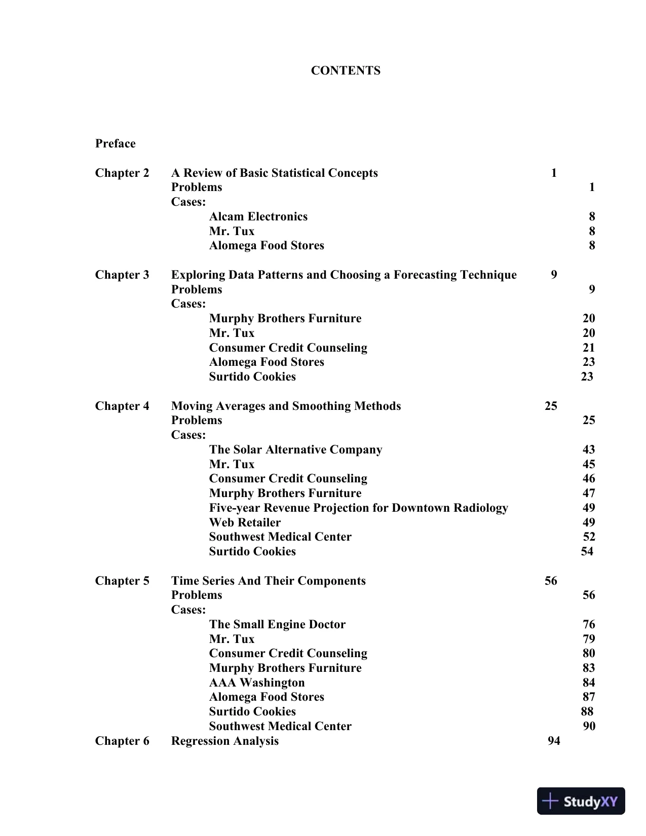
CONTENTSPrefaceChapter 2A Review of Basic Statistical Concepts1Problems1Cases:Alcam Electronics8Mr. Tux8Alomega Food Stores8Chapter 3Exploring Data Patterns and Choosing a Forecasting Technique9Problems9Cases:Murphy Brothers Furniture20Mr. Tux20Consumer Credit Counseling21Alomega Food Stores23Surtido Cookies23Chapter 4Moving Averages and Smoothing Methods25Problems25Cases:The Solar Alternative Company43Mr. Tux45Consumer Credit Counseling46Murphy Brothers Furniture47Five-year Revenue Projection for Downtown Radiology49Web Retailer49Southwest Medical Center52Surtido Cookies54Chapter 5Time Series And Their Components56Problems56Cases:The Small EngineDoctor76Mr. Tux79Consumer Credit Counseling80Murphy Brothers Furniture83AAA Washington84Alomega Food Stores87Surtido Cookies88Southwest Medical Center90Chapter 6Regression Analysis94
Page 2 of 31
Solution Manual for Business Forecasting, 9th Edition - Page 2 preview image
Page 3 of 31
Solution Manual for Business Forecasting, 9th Edition - Page 3 preview imageProblems94Cases:Tiger Transport Company113Butcher Products, Inc.113AceManufacturing114Mr. Tux114ConsumerCredit Counseling115AAA Washington117Chapter 7Multiple Regression120Problems120Cases:The Bond Market140AAA Washington141Fantasy Baseball (A)143Fantasy Baseball (B)145Chapter 8Regression With Time Series Data146Problems146Cases:Business Activity Index for Spokane County164Restaurant Sales165Mr. Tux165Consumer Credit Counseling166AAA Washington168Alomega Food Stores169Surtido Cookies169Southwest Medical Center171Chapter 9Box-Jenkins (ARIMA) Methodology173Problems173Cases:Restaurant Sales202Mr. Tux203Consumer Credit Counseling205The Lydia E. Pinkham Medicine Company207City of College Station209UPS Air Finance Division210AAA Washington212Web Retailer213Surtido Cookies215Southwest Medical Center218Chapter 10Judgmental Elements in Forecasting223Problems223
Page 4 of 31
Solution Manual for Business Forecasting, 9th Edition - Page 4 preview imageCases:Golden Gardens Restaurant224Alomega Food Stores224The Lydia E. Pinkham Medicine Company225Chapter 11Managing the Forecasting Process226Problems226Cases:Boundary Electronics226Busby Associates227Consumer Credit Counseling228Mr. Tux228Alomega Food Stores228Southwest Medical Center229
Page 5 of 31
Solution Manual for Business Forecasting, 9th Edition - Page 5 preview imagePREFACEThe goal of theninthedition of Business Forecasting remains the same as thatof the previous editions: To present the basic statistical techniques that are useful forpreparing individual business forecasts and long-range plans. This instructor’s manualcontains answers to chapter-end problems and comments on the case studies thatappear at the end of every chapter.Our work in forecasting over manyyears has taught us that intuition and goodjudgment are essential components of a good forecasting process, a point westress inChapters 1 and 11.This is a difficult concept to put across in the remaining chapters,which deal with important forecasting techniques involving data analysis.We hopethat the instructor can bring a measure of real-world common sense to the study offorecasting to supplement the quantitativematerial with which this instructor’s manualis concerned.We also hope that students can gain practical experience through hands on useof computer programs in their study of forecasting.Our solutions to problems andcases here rely heavily on Minitab software.Forecasters have just begun to tap thepotential offered by resources on the Internet.Data sets that appear in the text are available in several formats on the CDincluded with the book and on our website maintained by Prentice Hall atwww.prenhall.com/Hanke.Finally, we hope you find theninthedition ofBusiness Forecastinguseful.Comments for improvement are welcome. We can be reached at the following emailaddresses:John Hankejohn_hanke@msn.comDean Wichernd-wichern@tamu.edu
Page 6 of 31
Solution Manual for Business Forecasting, 9th Edition - Page 6 preview image1CHAPTER 2A REVIEW OF BASIC STATISTICAL CONCEPTSANSWERS TO PROBLEMS AND CASES1.Descriptive StatisticsVariableNMeanMedian StDev SE MeanOrders2821.3217.0013.372.53VariableMinMaxQ1Q3Orders5.0054.0011.2528.75a.X= 21.32b.S = 13.37c.S2= 178.76d.If the policy is successful, smaller orders will be eliminated and the mean willincrease.e.If the change causes all customers to consolidate a number of small orders intolarge orders, the standard deviation will probably decrease. Otherwise, it is verydifficult to tell how the standard deviation will be affected.f.The best forecast over the long-term is the mean of 21.32.2.Descriptive StatisticsVariableNMeanMedianStDevSE MeanPrices121766541800003944011385VariableMinMaxQ1Q3Prices121450253000138325205625X= 176,654andS = 39,4403.a.Point estimate:%76.10=Xb.1= .95Z= 1.96,n= 30,71.13,76.10==SX()()91.476.1030/71.1396.176.10/96.1==nSX(5.85%, 15.67%)c.df = 301 = 29,t= 2.045
Page 7 of 31
Solution Manual for Business Forecasting, 9th Edition - Page 7 preview image2()()12.576.1030/71.13045.276.10/045.2==nSX(5.64%, 15.88%)d.We see that the 95% confidence intervals inb and c are not much differentbecause the multipliers 1.96 and 2.045 are nearly the same magnitude.This explains why a sample of sizen= 30 is often taken as the cutoff betweenlarge and small samples.4.a.Point estimate:63259.10241.23=+=X95% error margin: (102.5923.41)/2 = 39.59b.1= .90Z= 1.645,2.2096.1/59.39/,63===nSX()23.3363)2.20(645.163/645.1==nSX(29.77, 96.23)5.H0:= 12.1n = 100= .05H1:> 12.1S = 1.7X= 13.5Reject H0if Z > 1.645Z =1007.11.125.13= 8.235Reject H0since the computed Z (8.235) is greater than the critical Z (1.645).The mean hasincreased.6.point estimate: 8.1 seatsinterval estimate: 8.11.96497.56.5 to 9.7 seatsForecast 8.1emptyseats per flight; very likely the meannumber of empty seatswill liebetween 6.5 and 9.7.7.n= 60,87.,60.5==SX9.5:9.5:10=HHtwo-sided test,= .05, critical value: |Z|= 1.96Test statistic:67.260/87.9.560.5/9.5===nSXZSince |2.67| = 2.67 > 1.96, reject0Hat the 5% level. The mean satisfaction rating isdifferent from 5.9.p-value: P(Z<2.67 orZ> 2.67) = 2 P(Z> 2.67) = 2(.0038) = .0076, very strongevidence against0H.
Page 8 of 31
Solution Manual for Business Forecasting, 9th Edition - Page 8 preview image38.df =n1 = 141 = 13,52.,31.4==SX4:4:10=HHone-sided test,= .05, critical value:t= 1.771Test statistic:23.214/52.431.4/4===nSXtSince 2.23 > 1.771, reject0Hat the 5% level. The medium-size serving contains anaverage of more than 4 ounces of yogurt.p-value: P(t> 2.23) = .022, strong evidence against0H9.H0:= 700n = 50= .05H1:700S = 50X= 715Reject H0if Z <-1.96 or Z > 1.96Z =5050700715= 2.12Since the calculated Z is greater than the critical Z (2.12 > 1.96), reject the null hypothesis.The forecast does not appear to be reasonable.p-value: P(Z<2.12 orZ> 2.12) = 2 P(Z> 2.12) = 2(.017) = .034, strong evidenceagainst0H10.This problem can be used to illustrate how a random sample is selected with Minitab. Inorder to generate 30 random numbers from a population of 200 click the following menus:Calc>Random Data>IntegerThe Integer Distribution dialog box shown in the figure belowappears. Thenumber ofrandom digits desired, 30, is entered in theNumber ofrows of datato generatespace. C1is entered forStore in column(s) and 1 and 200 are entered as the Minimum andMaximum values. OK is clicked and the 30 random numbers appear in Column 1 of theworksheet.
Page 9 of 31
Solution Manual for Business Forecasting, 9th Edition - Page 9 preview image4The null hypothesis that the mean is still 2.9 is true since the actual mean of thepopulation of data is 2.91 with a standard deviation of 1.608; however, a few students mayreject the null hypothesis, committing a Type I error.11.a.b.Positivelinear relationshipc.Y = 6058Y2= 4,799,724X = 59X2= 513XY = 48,665r = .938
Page 10 of 31
Solution Manual for Business Forecasting, 9th Edition - Page 10 preview image512.a.b.Positivelinear relationshipc.Y= 2312Y2= 515,878X = 53.7X2= 282.55XY = 12,029.3r = .95Yˆ= 32.5 + 36.4XYˆ= 32.5 + 36.4(5.2) = 22213.This is a good population for showing how random samples are taken. If three-digitrandom numbers are generated from Minitab as demonstrated in Problem 10, the selecteditems for the sample can be easily found. In this population,= 0.06somoststudentswillget a sample correlation coefficientrclose to 0. The least squares line will,inmost cases, have a slope coefficient close to 0,andstudents will not be able to reject thenull hypothesisH0: β1= 0 (or, equivalently, ρ = 0)if they carry out the hypothesis test.14.a.
Page 11 of 31
Solution Manual for Business Forecasting, 9th Edition - Page 11 preview image6b.Rent = 275.5 + .518 Sizec.Slope coefficient = .518Increase of $.518/month for each additional squarefoot of space.d.Size = 750Rent = 275.5 + .518(750) = $664/month15.n= 175,3.10,2.45==SXPoint estimate:2.45=X98% confidence interval: 1= .98Z= 2.33()()8.12.45175/3.1033.22.45/33.2==nSX(43.4, 47.0)Hypothesis test:44:44:10=HHtwo-sided test,= .02, critical value: |Z|= 2.33Test statistic:54.1175/3.10442.45/44===nSXZSince |Z| = 1.54 < 2.33, do not reject0Hat the 2% level.As expected, the results of the hypothesis test are consistentwith the confidenceinterval for;= 44 is not ruled out by either procedure.
Page 12 of 31
Solution Manual for Business Forecasting, 9th Edition - Page 12 preview image716.a.700,63:700,63:10=HHb.3.4:3.4:10=HHc.1300:1300:10=HH17.Large sample 95% confidence interval for mean monthly returnμ:)78.,98.2(88.110.13999.596.110.1=μ = .94 (%) is not a realistic value for mean monthly return of client’saccount since it falls outside the 95% confidence interval. Client may have acase.18.a.b.r= .581, positive linear association between wages and length of service.Other variables affecting wages may be size of bank and previous experience.c.WAGES= 324.3 + 1.006LOSWAGES= 324.3 + 1.006 (80) = 405
Page 13 of 31
Solution Manual for Business Forecasting, 9th Edition - Page 13 preview image8CASE 2-1: ALCAM ELECTRONICSIn our consulting work, business people sometimes tell us that business schools teach a risk-taking attitude that is too conservative. This is often reflected, we are told, in students choosing toolow a significance level: such a choice requires extreme evidence to move one from the status quo.This case can be used to generate a discussion on this point as David chooses= .01 and ends up"accepting" the null hypothesis that the mean lifetime is 5000 hours.Alice's point is valid: the company may be put in a bad position if it insists on very dramaticevidence before abandoning the notion that its components last 5000 hours. In fact, the indifference(p-value)is about .0375; at any higher level the null hypothesis of 5000 hours is rejected.CASE 2-2: MR. TUXIn this case, John Mosby tries some primitive ways of forecasting his monthly sales. Thethings he tries make some sort of sense, at least for a first cut, given that he has had no formaltraining in forecasting methods. Students should have no trouble finding flaws in his efforts, suchas:1.The mean value for each year, if projected into the future, is of little value sincemonth-to-month variability is missing.2.Hisfree-hand method of fitting a regression line through his data can be improveduponusing the least squares method, a technique now found on inexpensivehandcalculators. The large standard deviation for his monthly data suggestsconsiderable month-to-month variability and, perhaps,a strongseasonal effect, a factor not accounted for when the values for a year are averaged.Both the hand-fit regression line and John's interest in dealing with the monthly seasonalfactor suggest techniques to be studied in later chapters. His efforts also point out the value oflearning about well-established formal forecasting methods rather than relying on intuition andvery simple methods in the absence of knowledge about forecasting. We hope students will beginto appreciate the value of formal forecasting methods after learning about John's initial efforts.CASE 2-3: ALOMEGA FOOD STORESJulie’s initial look at her data using regression analysis is a good start. She found that ther-squared value of 36% is not very high. Using more predictor variables, along with examiningtheir significance in the equation, seems like a good next step. The case suggests that othertechniques may prove even more valuable, techniques to be discussed in the chapters that follow.Examining the residuals of her equation might prove useful. About how large are theseerrors? Are forecast errors in this range acceptable to her? Do the residuals seem to remain inthe same range over time, or do they increase over time?Are a string of negative residualsfollowed by a string of positive residuals or vice versa?These questions involve a deeperunderstanding of forecasting using historical values and these matters will be discussed morefully in later chapters.CHAPTER 3
Page 14 of 31
Solution Manual for Business Forecasting, 9th Edition - Page 14 preview image9EXPLORING DATA PATTERNS ANDCHOOSING A FORECASTING TECHNIQUEANSWERS TO PROBLEMS AND CASES1.Qualitative forecasting techniques rely on human judgment and intuition. Quantitativeforecasting techniques rely more on manipulation ofhistorical data.2.A time series consists of data that are collected, recorded, or observed over successiveincrements of time.3.The secular trend of a time series is the long-term component that represents the growth ordecline in the series over an extended period of time. The cyclical component is the wave-like fluctuation around the trend. The seasonal component is a pattern of change thatrepeats itself year after year. The irregular componentis that partof the timeseriesremainingafter the other components have been removed.4.Autocorrelation is the correlation between a variable, lagged one or more period, and itself.5.The autocorrelation coefficient measures the correlation between a variable, lagged one ormore periods, and itself.6.The correlogram is a useful graphical tool for displaying the autocorrelations for variouslags of a time series.Typically, the time lags are shown on a horizontal scale and theautocorrelation coefficients, thecorrelations between Ytand Yt-k,are displayed as verticalbars at the appropriate time lags. The lengths and directions (from 0) of the bars indicatethe magnitude and sign of theof the autocorrelation coefficients.The lags at whichsignificant autocorrelations occur provide information about the nature of the time series.7.a.nonstationary seriesb.stationary seriesc.nonstationary seriesd.stationary series8.a.stationary seriesb.random seriesc.trendingor nonstationary seriesd.seasonal seriese.stationary seriesf.trendingor nonstationary series9.Naive methods, simple averaging methods, moving averages,and Box-Jenkins methods.Examples are: the number of breakdowns per week on an assembly line having a uniformproduction rate; the unit sales of a product or service in the maturation stage of its life
Page 15 of 31
Solution Manual for Business Forecasting, 9th Edition - Page 15 preview image10cycle; and the number of sales resulting from a constant level of effort.10.Moving averages,simple exponential smoothing,Holt's linear exponential smoothing,simple regression, growth curves, and Box-Jenkins methods.Examples are: salesrevenues of consumer goods, demand for energy consumption, and use of raw materials.Other examples include: salaries,production costs, and prices, the growth period of thelife cycle of a new product.11.Classical decomposition, census II, Wintersexponential smoothing, time series multipleregression, and Box-Jenkins methods. Examples are: electrical consumption,summer/winter activities (sports like skiing), clothing, and agricultural growing seasons,retail sales influenced by holidays, three-day weekends, and school calendars.12.Classical decomposition, economic indicators, econometric models, multiple regression,and Box-Jenkins methods. Examples are: fashions, music, and food.13.19852,413-1999235811419862,407-620002329-2919872,403-4200123451619882,396-720022254-9119892,403720032245-919902,44340200422793419912,371-7219922,362-919932,334-2819942,3622819952,336-2619962,344819972,3844019982,244-140Yes! The original series has a decreasing trend.14.01.96 (180) = 01.96 (.1118) = 0.21915.a.MPEb.MAPEc.MSEor RMSE16.All four statements are true.17.a.r1= .895H0: ρ1= 0H1: ρ10
Page 16 of 31
Solution Manual for Business Forecasting, 9th Edition - Page 16 preview image11Reject if t <-2.069 or t > 2.069SE(kr) =nrkii=+11221=()242111121=+ir=241=.204)SE(rk11=rt=.2040895.= 4.39Since thecomputed t (4.39) is greater than the critical t (2.069), reject the null.r2= .788H0: ρ2= 0H1: ρ20Reject if t <-2.069 or t > 2.069SE(kr) =nrkii=+11221=()24895.211212=+i=2 624.= .33)SE(r111=rt=..788 033= 2.39Since the computed t (4.39) is greater than the critical t (2.069), reject the null.b.The data are nonstationary.See plot below.
Page 17 of 31
Solution Manual for Business Forecasting, 9th Edition - Page 17 preview image12The autocorrelation function follows.18.a.r1= .376b.The differenced data are stationary. See plot below.
Page 18 of 31
Solution Manual for Business Forecasting, 9th Edition - Page 18 preview image13The autocorrelation function follows.19.Figure 3-18-The data are nonstationary. (Trendingdata)Figure 3-19-The data are random.Figure 3-20-The data are seasonal. (Monthly data)Figure 3-21-The data are stationary and haveapattern that could be modeled.
Page 19 of 31
Solution Manual for Business Forecasting, 9th Edition - Page 19 preview image1420.The datahave aquarterlyseasonal patternas shown by the significant autocorrelationat time lag 4.First quarter earnings tend to be high,third quarter earnings tend to be low.
Page 20 of 31
Solution Manual for Business Forecasting, 9th Edition - Page 20 preview image15a.Time Data Forecast ErrortYtYˆtetetet2ttYettYe1.40------2.29.40-.11.11.0121.3793-.37933.24.29-.05.05.0025.2083-.20834.32.24.08.08.0064.2500.25005.47.32.15.15.0225.3191.31916.34.47-.13.13.0169.3824-.38247.30.34-.04.04.0016.1333-.13338.39.30.09.09.0081.2308.23089.63.39.24.24.0576.3810.381010.43.63-.20.20.0400.4651-.465111.38.43-.05.05.0025.1316-.131612.49.38.11.11.0121.2245.224513.76.49.27.27.0729.3553.355314.51.76-.25.25.0625.4902-.490215.42.51-.09.09.0081.2143-.214316.61.42.19.19.0361.3115.311517.86.61.25.25.0625.2907.290718.51.86-.35.35.1225.6863-.686319.47.51-.04.04.0016.0851-.085120.63.47.16.16.0256.2540.254021.94.63.31.31.0961.3298.329822.56.94-.38.38.1444.6786-.678623.50.56-.06.06.0036.1200-.120024.65.50.15.15.0225.2308.230825.95.65.30.30.0900.3158.315826.42.95-.53.53.28091.2619-1.261927.57.42.15.15.0225.2632.263228.60.57.03.03.0009.0500.050029.93.60.33.33.1089.3548.354830.38.93-.55.55.3025 1.4474-1.447431.37.38-.01.01.0001.0270-.027032.57.37.20.20.0400.3509.35095.851.686511.2227-2.1988b.MAD =3185.5= .189c.MSE =316865.1= .0544,RMSE = √.0544 =.2332
Page 21 of 31
Solution Manual for Business Forecasting, 9th Edition - Page 21 preview image16d.MAPE =312227.11= .3620or36.2%e.MPE =311988.2=-.070921.a.Time series plot followsb.The sales time series appears to vary about a fixed level so it is stationary.c.The sample autocorrelation function for the sales series follows:The sample autocorrelations die out rapidly. This behavior is consistent with astationary series. Note that the sales data are not random. Sales in adjacentweeks tend to be positively correlated.
Page 22 of 31
Solution Manual for Business Forecasting, 9th Edition - Page 22 preview image1722.a.The residualsYYett=are listed belowb.The residual autocorrelations followSince, in this case, the residuals differ from the original observations by theconstant05.2460=Y, the residual autocorrelations will be the same as theautocorrelations for the sales numbers. There is significant residualautocorrelation at lag 1 and the autocorrelations die out in an exponential fashion.The random model is not adequate for these data.23.a.& b.Time series plot follows.
Page 23 of 31
Solution Manual for Business Forecasting, 9th Edition - Page 23 preview image18Since this series is trending upward, it is nonstationary. There is also a seasonalpattern since 2ndand 3rdquarter earnings tend to be relatively large and 1stand 4thquarter earnings tend to be relatively small.c. The autocorrelation function for the first 10 lags follows.The autocorrelations are consistent with choice in part b. The autocorrelations failto die out rapidly consistent with nonstationary behavior. In addition, there arerelatively large autocorrelations at lags 4 and 8, indicating a quarterly seasonalpattern.
Page 24 of 31
Solution Manual for Business Forecasting, 9th Edition - Page 24 preview image1924.a. & b.Time series plotof fourth differencesfollows.The time series of fourth differences appears to be stationary as it variesabout a fixed level.25.a.98/99Inc98/99For98/99Err98/99AbsErr98/99Err^298/99AbE/Inc70.0150.8719.1419.14366.340.273390133.3993.8339.5639.561564.990.296574129.6492.5137.1337.131378.640.286409100.3880.5519.8319.83393.230.19754995.8570.0125.8425.84667.710.269588157.76133.3924.3724.37593.900.154475126.98129.64-2.662.667.080.02094893.80100.38-6.586.5843.300.070149Sum175.115015.171.5691b.MAD = 175.11/8 = 21.89,RMSE =√5015.17 = 70.82, MAPE = 1.5691/8 = .196or 19.6%c.Naïve forecasting method of part a assumes fourth differences are random.Autocorrelation function for fourth differences suggests they are not random.Error measures suggest naïve method not very accurate. In particular, on average,there is about a 20% error.However, naïve method does pretty well for 1999.Hard to think of another naïve method that will do better.
Page 25 of 31
Solution Manual for Business Forecasting, 9th Edition - Page 25 preview image20CASE 3-1A: MURPHY BROTHERS FURNITURE1.The retailsales series has a trend and a monthly seasonal pattern.2.Yes! Julie has determined that her data have a trend and should be first differenced. She hasalso found out that the first differenced data are seasonal.3.Techniques that she should consider includeclassical decomposition, Wintersexponential smoothing, time series multiple regression, and Box-Jenkins methods.4.She will know which technique works best by comparing error measurements such as MAD,MSEor RMSE, MAPE, and MPE.CASE 3-1B: MURPHY BROTHERS FURNITURE1.The retail sales series has a trend andamonthly seasonal pattern.2.The patterns appear to be somewhat similar. More actual data is needed in order toreachadefinitive conclusion.3.This question should create a lively discussion. There are good reasons to use either set ofdata. The retail sales series should probably be used until more actual sales data is available.CASE 3-2: MR. TUX1.This case affords students an opportunity to learn about the use ofautocorrelation functions,and tocontinue following John Mosby's quest to find a good forecasting method for hisdata.Withthe use of Minitab, the concept of first differencing data is also illustrated. Thesummary should conclude that the sales data have both a trend anda seasonal component.2.The trend is upward. Since there are significant autocorrelation coefficients at time lags 12and 24, the datahave a monthly seasonal pattern.3.There is a 49% random component. That is, about half the variability in John’s monthlysales is not accounted for by trend and seasonal factors. John, and the students analyzingthese results, should realize that finding an accurate method of forecasting these datacouldbe verydifficult.4.Yes, thefirst differences have a seasonal component. Given the autocorrelations at lags 12and 24, the monthly changes are related 12, 24, … months apart. This information should beused in developing a forecasting model forchanges in monthly sales.
Page 26 of 31
Solution Manual for Business Forecasting, 9th Edition - Page 26 preview image21CASE 3-3: CONSUMER CREDIT COUNSELING1.First, Dorothy used Minitab tocompute the autocorrelation function for the number of newclients. The results are shownbelow.221221.00.80.60.40.20.0-0.2-0.4-0.6-0.8-1.0LBQTCorrLagLBQTCorrLagLBQTCorrLagLBQTCorrLag165.14156.84153.39152.33148.66146.40144.86144.37138.70136.27134.55127.70121.68106.87100.7296.9093.7187.8781.6175.6067.1855.5142.8624.081.260.830.460.870.690.580.331.140.750.641.301.252.051.351.091.011.401.491.501.852.302.563.504.830.250.160.090.170.130.110.060.220.140.120.240.230.360.230.180.170.230.240.240.280.330.350.430.49242322212019181716151413121110987654321Autocorrelation Function for ClientsSince the autocorrelations failed to die out rapidly, Dorothy concluded her series wastrending or nonstationary. She then decided to difference her time series.
Page 27 of 31
Solution Manual for Business Forecasting, 9th Edition - Page 27 preview image22The autocorrelations for the first differenced series are:221221.00.80.60.40.20.0-0.2-0.4-0.6-0.8-1.0LBQTCorrLagLBQTCorrLagLBQTCorrLagLBQTCorrLag47.0042.0941.9340.0238.9838.9538.9334.8529.5229.3227.7226.2024.0719.6718.9118.9118.4918.3918.3417.8717.8317.8217.6617.431.44-0.26-0.920.69-0.110.09-1.411.67-0.32-0.930.92-1.111.65-0.690.02-0.520.260.17-0.570.170.10-0.330.41-4.110.19-0.03-0.120.09-0.020.01-0.180.21-0.04-0.120.11-0.140.20-0.080.00-0.060.030.02-0.070.020.01-0.040.05-0.42242322212019181716151413121110987654321Autocorrelations for Differenced Data2.The differences appear to be stationary and are correlated in consecutive time periods.Giventhe somewhat large autocorrelations at lags 12 and 24, a monthly seasonal pattern should beconsidered.3.Dorothy would recommend that various seasonal techniques such as Wintersmethod ofexponential smoothing (Chapter 4), classical decomposition (Chapter 5), time seriesmultiple regression (Chapter 8)andBox-Jenkins methods (ARIMA models inChapter 9) beconsidered.
Page 28 of 31
Solution Manual for Business Forecasting, 9th Edition - Page 28 preview image23CASE 3-4:ALOMEGA FOOD STORESThe sales data from Chapter 1 for the Alomega Food Stores case are reprinted in Case3-4. The case suggests that Julie look at the data pattern for hersales data.The autocorrelationfunction for sales follows.Autocorrelations suggest an up and down pattern thatis very regular. If one month isrelatively high, next month tends to be relatively low and so forth. Very regularpattern is suggested by persistence of autocorrelations at relatively large lags.The changing ofthesignof the autocorrelations from one lag to the next is consistent withan up and down pattern in the time series. If high sales tend to be followed by low sales orlow sales by high sales, autocorrelations at odd lags will be negative and autocorrelations ateven lags positive.Therelatively large autocorrelation atlag 12, 0.53, suggests there may also be a seasonalpattern. This issue is explored in Case 5-6.CASE 3-5: SURTIDO COOKIES1.A time series plot and the autocorrelation function for Surtido Cookies sales follow.
Page 29 of 31
Solution Manual for Business Forecasting, 9th Edition - Page 29 preview image24The graphical evidence above suggests Surtido Cookies sales vary about a fixed level witha strong monthly seasonal component. Sales are typically high near the end of the year andlow during the beginning of the year.2.03SalesNaiveForErrAbsErrAbsE/03SalesMAD = 678369/5 = 13567410726176811173915003915000.364995MAPE = .816833/5 =.163 or 16.3%510005549689-39684396840.07781157954149705982482824820.1423237713506524491189011189010.154147590556636358-45802458020.077557Sum6783690.816833MAD appears large because of the big numbers for sales. MAPE is fairly large butperhaps tolerable. In any event, Jame is convinced he can do better.
Page 30 of 31
Solution Manual for Business Forecasting, 9th Edition - Page 30 preview image25CHAPTER 4MOVING AVERAGES AND SMOOTHING METHODSANSWERS TO PROBLEMS AND CASES1.Exponential smoothing2.Naive3.Moving average4.Holt's two-parametersmoothing procedure5.Wintersthree-parametersmoothing procedure6.a.tYttYˆetetet2ttYettYe119.3919.00.39.39.1521.020.020218.9619.39-.43.43.1849.023-.023318.2018.96-.76.76.5776.042-.042417.8918.20-.31.31.0961.017-.017518.4317.89.54.54.2916.029.029619.9818.431.551.552.4025.078.078719.5119.98-.47.47.2209.024-.024820.6319.511.121.121.2544.054.054919.7820.63-.85.85.7225.043-.0431021.2519.781.471.47 2.1609.069.0691121.1821.25-.07.07.0049.003-.0031222.1421.18.96.96.9216.043.0438.928.990.445.141b.MAD =1292.8= .74c.MSE =8 9912.= .75
Page 31 of 31
Solution Manual for Business Forecasting, 9th Edition - Page 31 preview image26d.MAPE =.44512= .0371e.MPE =.14112= .0118f.22.147.PriceAVER1FITS1RESI119.39***18.96***18.2018.8500**17.8918.350018.8500-0.9600018.4318.173318.35000.0800019.9818.766718.17331.8066719.5119.306718.76670.7433320.6320.040019.30671.3233319.7819.973320.0400-0.2600021.2520.553319.97331.2766721.1820.736720.55330.6266722.1421.523320.73671.40333Accuracy MeasuresMAPE: 4.6319MAD: 0.9422MSE: 1.1728The naïve approach is better.8.a.See plot below.YtAvgFitsRes200***210***215***216***219212**22021621282252192169226221.22197221.2Accuracy MeasuresMAPE: 3.5779MAD:8.0000MSE: 64.6667221.2 is forecast for period 9
Preview Mode

This document has 234 pages. Sign in to access the full document!