Solution Manual for Introductory Econometrics: A Modern Approach, 5th Edition

Preview (31 of 279 Pages)

100%

Solution Manual for Introductory Econometrics: A Modern Approach, 5th Edition - Page 1 preview image

Loading page ...

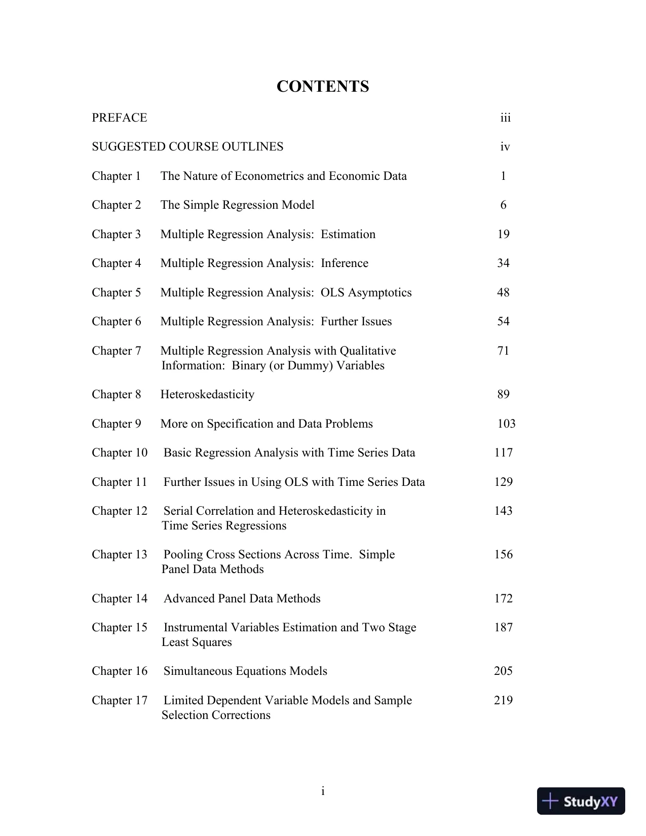
iCONTENTSPREFACEiiiSUGGESTED COURSE OUTLINESivChapter 1TheNature of Econometrics and Economic Data1Chapter 2The Simple Regression Model6Chapter 3Multiple Regression Analysis: Estimation19Chapter 4Multiple Regression Analysis: Inference34Chapter 5Multiple Regression Analysis: OLS Asymptotics48Chapter 6Multiple Regression Analysis: Further Issues54Chapter 7Multiple Regression Analysiswith Qualitative71Information: Binary (or Dummy) VariablesChapter 8Heteroskedasticity89Chapter 9More on Specification and Data Problems103Chapter 10Basic Regression Analysiswith Time Series Data117Chapter 11Further Issues in Using OLSwith Time Series Data129Chapter 12Serial Correlation and Heteroskedasticity in143Time Series RegressionsChapter 13Pooling Cross Sections Across Time.Simple156Panel Data MethodsChapter 14Advanced Panel Data Methods172Chapter 15Instrumental Variables Estimation and Two Stage187Least SquaresChapter 16Simultaneous Equations Models205Chapter 17Limited Dependent Variable Models and Sample219Selection Corrections

Solution Manual for Introductory Econometrics: A Modern Approach, 5th Edition - Page 2 preview image

Loading page ...

Solution Manual for Introductory Econometrics: A Modern Approach, 5th Edition - Page 3 preview image

Loading page ...

iiChapter 18Advanced Time Series Topics243Chapter 19Carrying Out an Empirical Project259Appendix ABasic Mathematical Tools260Appendix BFundamentals of Probability263Appendix CFundamentals of Mathematical Statistics265Appendix DSummary of Matrix Algebra269Appendix EThe Linear Regression Model in Matrix Form271

Solution Manual for Introductory Econometrics: A Modern Approach, 5th Edition - Page 4 preview image

Loading page ...

iiiPREFACEThis manual contains suggested course outlines, teaching notes, and detailed solutions to all ofthe problems and computer exercises inIntroductory Econometrics: A Modern Approach,5e.For several problems,I have added additional notes about interesting asides or suggestions forhow to modify or extend the problem.Some of the answers given here are subjective, and you may want to supplement or replace themwith your own answers.I wrote all solutions as if I were preparing them for the students, so youmay find some solutions a bit tedious(if notbordering on an insult to your intelligence).Thisway, if you prefer, you can distribute my answers to some of the even-numbered problemsdirectly to the students.(The student study guide contains answers to all odd-numberedproblems.)Many of the equations in the Word files were created using MathType, and theequations will not look quite right without MathType.Some equations I have created using theequation editor in Word 2007.I solved thecomputer exercisesusing various versions ofStata, starting with version 4.0 andrunning through version12.0.Nevertheless, almost all of the estimation methods covered in thetext have been standardized, and different econometrics or statistical packages should give thesame answers. There can be differences when applying more advanced techniques, asconventions sometimes differ on how to choose orestimate auxiliary parameters.(Examplesinclude heteroskedasticity-robust standard errors, estimates of a random effects model, andcorrections for sample selection bias.)While I have endeavored to make the solutions mistake-free, some errors may have crept in. Iwould appreciate hearing from you if you find mistakes.I will update the manual occasionallyand correct any mistakes that have been found.I heard from many of you regarding theearliereditionsof the text, and I incorporated many of your suggestions. I welcome any comments thatwill help me make improvements to future editions. I can be reached via e-mail atwooldri1@.msu.edu.The fifth edition of the text drops the chapter numbers preceding the problems and computerexercises. I have kept the chapter numbers in the solutions manual so that it is easy to keep trackof where one is. For example, the solution to problem 4 in chapter 3 is labeled 3.4and computerexercise 6 in chapter 8 is labeled C8.6.I hope you find this instructor’s manual useful, and I look forward to hearing your reactions tothefifthedition.Jeffrey M. WooldridgeDepartment of EconomicsMichigan State University486 W. Circle Drive110 Marshall-Adams HallEast Lansing, MI 48824-1038

Solution Manual for Introductory Econometrics: A Modern Approach, 5th Edition - Page 5 preview image

Loading page ...

ivSUGGESTED COURSE OUTLINESFor an introductory, one-semester course, I like to cover most of the material in Chapters 1through 8 and Chapters 10 through 12, as well as parts of Chapter 9 (but mostly throughexamples). I do not typically cover all sections or subsections within each chapter. Under thechapter headings listed below, I provide some comments on the material I find most relevant fora first-semester course.An alternative course ignores time series applications altogether, while delving into some of themore advanced methods that are particularly useful for policy analysis. This would consist ofChapters 1 through 8, much of Chapter 9, and the first four sections of Chapter 13. Chapter 9discusses thepracticallyimportant topics of proxy variables, measurement error, outlyingobservations, and stratified sampling. In addition, I have written a more careful description ofthe method of least absolute deviations, including a discussion of its strengths and weaknesses.Chapter 13 covers, in a straightforward fashion, methods for pooled cross sections (including theso-called “natural experiment” approach) and two-period panel data analysis. The basic cross-sectional treatment of instrumental variables in Chapter 15 is a natural topic for cross-sectional,policy-oriented courses. For an accelerated course, the nonlinear methods used for cross-sectional analysis in Chapter 17 can be covered.I typically do not begin with a review ofbasic algebra, probability, and statistics. In myexperience, this takes too long and the payoff is minimal.(Students tend to think that they aretaking another statistics courseand start to drift away from the material.)Instead, when I need atool (such as the summation or expectations operator), I briefly review the necessary definitionsand key properties.Statistical inference is not more difficult to describe inthe context ofmultipleregression than in testing about mean a mean from apopulation, and so I briefly review theprinciples of statistical inference duringmultiple regression analysis.Appendices A,B, and C arefairly extensive.When I cover asymptotic properties of OLS, I provide a brief discussion of themain definitions andlimit theorems.If students need more than the brief review provided inclass, I point them to the appendices.For a master’s level course, I include a couple of lectures on the matrixapproach to linearregression.This could be integrated into Chapters 3 and4 or covered after Chapter 4.Again, I donot summarize matrix algebra before proceeding.Instead, the material in Appendix D can bereviewed as it is needed in covering Appendix E.A second semester course, at either the undergraduate or master’s level, could begin with someof the material in Chapter 9, particularly with the issues of proxy variables and measurementerror. Least absolute deviations and, more generally, quantile regression are used more and morein empirical work, and the fifth edition has sections that can be used as an introduction toquantile regression.The advanced chapters, starting with Chapter 13, areparticularlyuseful forstudentswithan interest in policy analysis.The pooled cross section and panel data chapters(Chapters 13 and 14) emphasize how these datastructurescan be used, in conjunction witheconometric methods, for policy evaluation.Chapter 15, which introduces the method ofinstrumental variables, is also important for policy analysis. Most modern IV applications areused to address the problems of omitted variables (unobserved heterogeneity) or measurement

Solution Manual for Introductory Econometrics: A Modern Approach, 5th Edition - Page 6 preview image

Loading page ...

verror.I have intentionally separated out the conceptually more difficult topic of simultaneousequations models in Chapter 16.Chapter 17, in particular the material on probit, logit, Tobit, and Poisson regression models, is agood introduction tononlinear econometric methods.Specialized courses that emphasizeapplications in labor economics can use the material on sample selection corrections. Durationmodels are also briefly covered as an example of a censored regression model.Chapter 18 is much different from the other advanced chapters, as it focuses on more advancedor recent developments in time series econometrics.Combined with some of the more advancedtopics in Chapter 12, it can serve as the basis for a second semester course in time series topics,including forecasting.Most second semester courses would include an assignment to write an original empirical paper,and Chapter 19 should be helpful in this regard.

Solution Manual for Introductory Econometrics: A Modern Approach, 5th Edition - Page 7 preview image

Loading page ...

1CHAPTER 1TEACHING NOTESYou have substantial latitude about what to emphasize in Chapter 1.I find it useful to talk aboutthe economics of crime example (Example 1.1) and the wage example (Example 1.2) so thatstudents see, at the outset, that econometrics is linked to economic reasoning,even if theeconomics is not complicatedtheory.I like to familiarize students with the important data structures that empirical economists use,focusing primarily on cross-sectional and time series data sets, as these are what I cover in afirst-semester course.It is probably a good idea to mention the growing importance of data setsthat have both a cross-sectional and time dimension.I spend almost an entire lecture talking about the problems inherent in drawing causal inferencesin the social sciences.I do this mostly through the agricultural yield, return toeducation, andcrime examples.These examples also contrast experimental and nonexperimental(observational)data.Students studying business and finance tend to find the term structure of interest ratesexample more relevant, although the issue there is testing the implication of a simple theory, asopposed to inferring causality.I have found that spending time talking about these examples, inplace of a formal review of probability and statistics, is more successfulin teaching the studentshow econometrics can be used.(And, it ismore enjoyable for the students and me.)I do not use counterfactual notation as in the modern “treatment effects” literature, but I dodiscuss causalityusing counterfactual reasoning. The return to education, perhaps focusing onthe return to getting a college degree, is a good example of how counterfactual reasoning iseasily incorporated into the discussion of causality.

Solution Manual for Introductory Econometrics: A Modern Approach, 5th Edition - Page 8 preview image

Loading page ...

2SOLUTIONS TO PROBLEMS1.1(i) Ideally, we could randomly assign studentsto classes of different sizes.That is, eachstudent is assigned a different class size without regard to any student characteristics such asability and family background.For reasons we will see in Chapter 2, we would like substantialvariation in class sizes (subject, of course, to ethical considerations and resource constraints).(ii) A negative correlation means that larger class size is associated with lower performance.We might find a negative correlation because larger class size actually hurts performance.However, with observational data, there are other reasons we might find a negative relationship.For example, children from more affluent families might be more likely to attend schools withsmaller class sizes, and affluent children generally score better on standardized tests. Anotherpossibility is that, within a school, a principal might assign the better students to smaller classes.Or, some parents might insist their children are in the smaller classes, and these same parentstend to be more involved in their children’s education.(iii) Given the potential for confounding factors–some of which are listed in (ii)–finding anegative correlation would not be strong evidence that smaller class sizes actually lead to betterperformance.Some way of controlling for the confounding factors is needed, and this is thesubject of multiple regression analysis.1.2(i)Here is one way to pose the question:If two firms, sayAandB, are identical in allrespects except that firmAsupplies job training one hour per worker more than firmB, by howmuch would firmA’s output differ from firmB’s?(ii)Firms are likely to choose job training depending on the characteristics of workers. Someobserved characteristics are years of schooling, years in the workforce, and experience in aparticular job. Firms might even discriminate based onage,gender,or race.Perhaps firmschoose to offer training to more or less able workers, where “ability” might be difficult toquantify but where a manager has some idea about therelative abilitiesof different employees.Moreover, different kinds of workers might be attracted to firms that offer more job training onaverage, and this might not be evident to employers.(iii) The amount of capital and technology available to workers would also affect output.So,two firms with exactly the same kinds of employees would generally have different outputs ifthey use different amounts of capital or technology.The quality of managers would also have aneffect.(iv)No, unless theamount of training is randomly assigned. The many factors listed in parts(ii) and (iii) can contribute to finding a positive correlation betweenoutputandtrainingeven ifjob training does not improve worker productivity.1.3It does not make sense topose thequestion in terms of causality.Economists would assumethat students choose a mix of studying and working(and other activities, such as attending class,leisure,and sleeping)based on rational behavior, such as maximizing utility subject to theconstraint that there are only168 hoursin a week.We can then use statistical methods to

Solution Manual for Introductory Econometrics: A Modern Approach, 5th Edition - Page 9 preview image

Loading page ...

3measure the association between studying and working, including regression analysis, whichwecover starting in Chapter 2.But we would not be claiming that one variable “causes” the other.They are both choice variables of the student.SOLUTIONS TO COMPUTER EXERCISESC1.1(i) The average ofeducis about 12.6 years.There are two people reporting zero years ofeducation, and 19 people reporting 18 years of education.(ii)The average ofwageis about $5.90, whichseems low inthe year2008.(iii)Using TableB-60in the 2004Economic Report of thePresident,the CPIwas56.9in1976 and184.0in 2003.(iv) To convert 1976 dollars into 2003 dollars, we use the ratio of the CPIs, which is184/ 56.93.23. Therefore, the average hourly wage in 2003dollars isroughly3.23($5.90)$19.06, which is a reasonable figure.(v)The sample contains252 women (the number of observations withfemale= 1) and 274men.C1.2(i)There are 1,388 observations in the sample.Tabulating the variablecigsshows that 212women havecigs> 0.(ii)The average ofcigsis about 2.09, but this includesthe 1,176 women who did notsmoke. Reporting just the average masks the fact that almost 85 percent of the women did notsmoke.It makes more sense to say that the “typical” womandoes not smoke during pregnancy;indeed, the mediannumber of cigarettes smoked is zero.(iii) The average ofcigsover the women withcigs> 0 is about 13.7. Of course this ismuch higher than the average over the entire sample because we are excluding 1,176 zeros.(iv) The average offatheducis about 13.2. There are 196 observations with a missingvalue forfatheduc, and those observations are necessarily excluded in computing the average.(v) The average and standard deviation offamincare about29.027 and18.739,respectively, butfamincis measured in thousands of dollars. So, in dollars, the average andstandard deviation are$29,027 and $18,739.C1.3(i)The largest is 100,thesmallest is 0.(ii) 38out of 1,823, or about 2.1 percent of the sample.(iii)17

Solution Manual for Introductory Econometrics: A Modern Approach, 5th Edition - Page 10 preview image

Loading page ...

4(iv) The average ofmath4is about 71.9 and the average ofread4is about 60.1. So, at leastin 2001, the reading test was harder to pass.(v) The sample correlation betweenmath4andread4is about .843, which is a very highdegree of (linear) association. Not surprisingly, schools that have high pass rates on one testhave a strong tendency tohave highpass rates on the other test.(vi) The average ofexpppis about $5,194.87. Thestandard deviationis$1,091.89, whichshows rather wide variation in spending per pupil. [The minimum is$1,206.88andthemaximumis$11,957.64.](vii)The percentage by which school A outspends school Bis100∙(6,000−5,500)5,500≈9.09%When we use the approximation based on the difference of the natural logs we geta somewhatsmaller number:100∙[log(6,000)−log(5,500)]≈8.71%C1.4(i)185/445.416 is the fraction of men receiving job training, or about 41.6%.(ii)For men receiving job training, the average ofre78is about6.35, or $6,350. For men notreceiving job training, the average ofre78is about4.55, or $4,550. The difference is $1,800,which is very large. On average, the men receiving the job training had earnings about 40%higher than those not receiving training.(iii)About 24.3% of the men who received training were unemployed in 1978; the figure is35.4% for men not receiving training. This, too, is a big difference.(iv)Thedifferences in earnings and unemployment rates suggest the training program hadstrong, positive effects. Our conclusions about economic significance would be stronger if wecould also establish statistical significance (which is done in Computer Exercise C9.10 inChapter 9).C1.5(i) The smallest and largest values ofchildrenare 0 and 13, respectively. The average isabout 2.27.(ii) Out of4,358women, only 611 have electricity in the home, or about 14.02 percent.(iii)The average ofchildrenfor women without electricity is about 2.33, and for those withelectricity it is about 1.90. So, on average, women with electricity have .43 fewer children thanthose who do not.(iv) We cannot infer causality here. There are many confounding factors that may be relatedto the number of children and the presence of electricity in the home; household income andlevel of education are two possibilities. For example, it could be that women with more

Solution Manual for Introductory Econometrics: A Modern Approach, 5th Edition - Page 11 preview image

Loading page ...

5education have fewer children and are more likely to have electricity in the home (the latter dueto an income effect).

Solution Manual for Introductory Econometrics: A Modern Approach, 5th Edition - Page 12 preview image

Loading page ...

6CHAPTER 2TEACHING NOTESThis is the chapter where I expect students to follow most, if not all,of the algebraic derivations.In class I like to derive at least the unbiasedness of the OLS slope coefficient, and usually Iderive the variance.At a minimum, I talk about the factors affecting the variance.To simplifythe notation, after I emphasize the assumptions in the population model, and assume randomsampling, I just condition on the values of the explanatory variables in the sample. Technically,this is justified by random sampling because, for example, E(ui|x1,x2,…,xn) = E(ui|xi) byindependent sampling.I find that students are able to focus on the key assumption SLR.4 andsubsequently take my word about how conditioning on the independent variables in the sample isharmless.(If you prefer, the appendix to Chapter 3 does the conditioning argument carefully.)Because statistical inference is no more difficult in multiple regression than in simple regression,I postpone inference until Chapter 4.(This reduces redundancy and allows you to focus on theinterpretive differences between simple and multiple regression.)You might notice how, compared with most other texts, I use relatively few assumptions toderive the unbiasedness of the OLS slope estimator, followed by the formula for its variance.This is because I do not introduce redundant or unnecessary assumptions.For example, onceSLR.4is assumed, nothing further about the relationship betweenuandxis needed to obtain theunbiasedness of OLS under random sampling.Incidentally,one of the uncomfortable facts aboutfinite-sample analysis is that there is adifference between an estimator that is unbiased conditional on the outcome of the covariates andone that is unconditionally unbiased. If the distribution of the𝑥𝑖is such that they can all equalthe same value with positive probability–as is the case with discreteness in the distribution–then the unconditional expectation does not really exist. Or, if it is made to exist then theestimator is not unbiased. I do not try to explain these subtleties in an introductory course, but Ihave had instructors ask me about the difference.

Solution Manual for Introductory Econometrics: A Modern Approach, 5th Edition - Page 13 preview image

Loading page ...

7SOLUTIONS TO PROBLEMS2.1(i) Income, age, and family background (such as number of siblings) are just a fewpossibilities. It seems that each of these could be correlated with years of education. (Incomeand education are probably positively correlated; age and education may be negatively correlatedbecause women in more recent cohorts have, on average, more education; and number of siblingsand education are probably negatively correlated.)(ii) Not if the factors we listed in part (i) are correlated witheduc. Because we would like tohold these factors fixed, they are part of the error term. But ifuis correlated witheducthenE(u|educ)0, and so SLR.4fails.2.2In the equationy=0+1x+u, add and subtract0from the right hand side to gety= (0+0) +1x+ (u−0). Call the new errore=u−0, so that E(e)= 0. The new intercept is0+0, but the slope is still1.2.3(i) Letyi=GPAi,xi=ACTi, andn= 8. Thenx= 25.875,y= 3.2125,1ni=(xi–x)(yi–y)=5.8125, and1ni=(xi–x)2= 56.875. From equation (2.9), we obtain the slope as1ˆ=5.8125/56.875.1022, rounded to four places after the decimal. From (2.17),0ˆ=y–1ˆx3.2125–(.1022)25.875.5681. So we can writeGPA= .5681 + .1022ACTn= 8.The intercept does not have a useful interpretation becauseACTis not close to zero for thepopulation of interest. IfACTis 5 points higher,GPAincreases by .1022(5)= .511.(ii) The fitted values and residuals—rounded to four decimal places—are given along withthe observation numberiandGPAin the following table:

Solution Manual for Introductory Econometrics: A Modern Approach, 5th Edition - Page 14 preview image

Loading page ...

8iGPAGPAˆu12.82.7143.085723.43.0209.379133.03.2253–.225343.53.3275.172553.63.5319.068163.03.1231–.123172.73.1231–.423183.73.6341.0659You can verify that the residuals, as reported in the table, sum to−.0002, which is pretty close tozero given the inherent rounding error.(iii) WhenACT= 20,GPA= .5681 + .1022(20)2.61.(iv) The sum of squared residuals,21ˆniiu=, is about .4347 (rounded to four decimal places),and the total sum of squares,1ni=(yi–y)2, is about 1.0288.So theR-squared from the regressionisR2= 1–SSR/SST1–(.4347/1.0288).577.Therefore, about 57.7% of the variation inGPAis explained byACTin this small sample ofstudents.2.4(i) Whencigs= 0, predicted birth weight is 119.77 ounces. Whencigs= 20,bwght= 109.49.This is about an 8.6% drop.(ii) Not necessarily. There are many other factors that can affect birth weight, particularlyoverall health of the mother and quality of prenatal care.These could be correlated withcigarette smoking during birth. Also, something such as caffeine consumption can affect birthweight, and might also be correlated with cigarette smoking.(iii) If we want a predictedbwghtof 125, thencigs= (125–119.77)/(–.524)–10.18, orabout–10 cigarettes! This is nonsense, of course, and it shows what happens when we are tryingto predict something as complicated as birth weight with only a single explanatory variable. Thelargest predicted birth weight is necessarily 119.77. Yet almost 700 of the births in the samplehad a birth weight higher than 119.77.

Solution Manual for Introductory Econometrics: A Modern Approach, 5th Edition - Page 15 preview image

Loading page ...

9(iv) 1,176 out of 1,388 women did not smoke while pregnant, or about 84.7%. Because weare using onlycigsto explain birth weight, we have only one predicted birth weight atcigs= 0.The predicted birth weight is necessarily roughly in the middle of the observed birth weights atcigs= 0, and so we will under predict high birth rates.2.5(i) The intercept implies that wheninc= 0,consis predicted to be negative $124.84. This, ofcourse, cannot be true, and reflects that fact that this consumption function might be a poorpredictor of consumption at very low-income levels. On the other hand, on an annual basis,$124.84 is not so far from zero.(ii) Just plug 30,000 into the equation:cons=–124.84 + .853(30,000)= 25,465.16 dollars.(iii) The MPC and the APC are shown in the following graph. Even though the intercept isnegative, the smallest APC in the sample is positive. The graph starts at an annual income levelof $1,000 (in 1970 dollars).2.6(i) Yes. If living closer to an incinerator depresses housing prices, then being farther awayincreases housing prices.(ii) If the city chose to locate the incinerator in an area away from more expensiveneighborhoods, then log(dist) is positively correlated with housing quality. This would violateSLR.4, and OLS estimation is biased.inc1000100002000030000.7.728.853APCMPC.9APCMPC

Solution Manual for Introductory Econometrics: A Modern Approach, 5th Edition - Page 16 preview image

Loading page ...

10(iii) Size of the house, number of bathrooms, size of the lot, age of the home, and quality ofthe neighborhood (including school quality), are just a handful of factors. As mentioned in part(ii), these could certainly be correlated withdist[and log(dist)].2.7(i) When we condition onincin computing an expectation,incbecomes a constant. SoE(u|inc)= E(ince|inc) =incE(e|inc)=inc0 because E(e|inc)= E(e)= 0.(ii) Again, when we condition onincin computing a variance,incbecomes a constant. SoVar(u|inc)= Var(ince|inc)= (inc)2Var(e|inc)=2eincbecause Var(e|inc)=2e.(iii) Families with low incomes do not have much discretion about spending; typically, alow-income family must spend on food,clothing, housing, and other necessities. Higher incomepeople have more discretion, and some might choose more consumption while others moresaving. This discretion suggests wider variability in saving among higher income families.2.8(i) From equation (2.66),1=1niiix y=/21niix=.Plugging inyi=0+1xi+uigives1=011()niiiixxu=++/21niix=.After standard algebra, thenumerator can be written as201111innniiiiiixxx u===++.Putting this over the denominator shows we can write1as1=01niix=/21niix=+1+1niiix u=/21niix=.Conditional on thexi, we haveE(1) =01niix=/21niix=+1

Solution Manual for Introductory Econometrics: A Modern Approach, 5th Edition - Page 17 preview image

Loading page ...

11because E(ui) = 0 for alli. Therefore, the bias in1is given by the first term in this equation.This bias is obviously zero when0= 0. It is also zero when1niix== 0, which is the same asx= 0. In the latter case, regression through the origin is identical to regression with an intercept.(ii) From the last expression for1in part (i) we have, conditional on thexi,Var(1)=221niix−=Var1niiix u==221niix−=21Var()niiixu==221niix−=221niix==2/21niix=.(iii) From (2.57), Var(1ˆ) =2/21()niixx=−. From the hint,21niix=21()niixx=−, and soVar(1)Var(1ˆ). A more direct way to see this is to write21()niixx=−=221()niixn x=−, whichis less than21niix=unlessx= 0.(iv) Fora given sample size, the bias in1increases asxincreases (holding the sum of the2ixfixed). But asxincreases, the variance of1ˆincreases relative to Var(1). The bias in1is also small when0is small. Therefore, whether we prefer1or1ˆon a mean squared errorbasis depends on the sizes of0,x, andn(in addition to the size of21niix=).2.9(i) We follow the hint, noting that1c y=1c y(the sample average of1ic yisc1times thesample average of yi) and2c x=2c x. When we regressc1yionc2xi(including an intercept) weuse equation (2.19) to obtain the slope:2211121112222221111112221()()()()()()()()ˆ.()nniiiiiinniiiiniiiniic xc xc yc yc cxxyyc xc xcxxxxyyccccxx======−−−−==−−−−==−

Solution Manual for Introductory Econometrics: A Modern Approach, 5th Edition - Page 18 preview image

Loading page ...

12From (2.17), we obtain the intercept as0= (c1y)–1(c2x)= (c1y)–[(c1/c2)1ˆ](c2x)=c1(y–1ˆx)=c10ˆ) because the intercept from regressing yion xiis (y–1ˆx).(ii) We use the same approach from part (i) along with the fact that1()cy+=c1+yand2()cx+=c2+x. Therefore,11()()icycy+−+= (c1+yi)–(c1+y)=yi–yand (c2+xi)–2()cx+=xi–x. Soc1andc2entirely drop out of the slope formula for the regression of (c1+yi) on (c2+xi), and1=1ˆ. The intercept is0=1()cy+–12()cx+= (c1+y)–1ˆ(c2+x)= (1ˆyx−)+c1–c21ˆ=0ˆ+c1–c21ˆ, which is what we wanted to show.(iii) We can simply apply part (ii) because11log()log()log()iic ycy=+. In other words,replacec1with log(c1),yiwith log(yi), and setc2= 0.(iv) Again, we can apply part (ii) withc1= 0 and replacingc2with log(c2) andxiwith log(xi).If01ˆˆandare the original intercept and slope, then11ˆ=and0021ˆˆlog()c=−.2.10(i) Thisderivation is essentially donein equation (2.52), once(1/ SST )xis brought insidethe summation (which is valid becauseSSTxdoes not depend oni).Then, just define/ SSTiixwd=.(ii) Because111ˆˆCov(,)E[() ] ,uu=−we show that the latter is zero. But, from part (i),()1111ˆE[()] =EE().nniiiiiiuw uuwu u==−=Because theiuare pairwiseuncorrelated(they are independent),22E()E(/)/iiu uunn==(becauseE()0,ihu uih=).Therefore,(iii)The formula for the OLS intercept is0ˆˆyx=−and, plugging in01yxu=++gives0011011ˆˆˆ()() .xuxux=++−=+−−(iv)Because1ˆanduare uncorrelated,222222201ˆˆVar()Var( )Var()/(/ SST )// SSTxxuxnxnx=+=+=+,which is what we wanted to show.(v) Using the hint and substitution gives()220ˆVar()[ SST /]/ SSTxxnx=+()()2122221211/ SST/ SST .nnixixiinxxxnx−−===−+=22111E()(/)(/)0.nnniiiiiiiwu uwnnw======

Solution Manual for Introductory Econometrics: A Modern Approach, 5th Edition - Page 19 preview image

Loading page ...

132.11(i) We would want to randomly assign the number of hours in the preparation course so thathoursisindependent of other factors that affect performance on the SAT. Then, we wouldcollect information on SAT score for each student in the experiment, yielding a data set{(,) :1,..., }iisathoursin=, wherenis the number of students we can afford to have in the study.From equation (2.7), we should try to get as much variation inihoursas is feasible.(ii)Here are three factors: innate ability, family income, andgeneral health on the day of theexam. If we think students with higher native intelligence think they do not need to prepare forthe SAT, then ability andhourswill be negatively correlated. Family income would probably bepositively correlated withhours, because higher income families can more easily affordpreparation courses. Ruling out chronic health problems, health on the day of the exam shouldbe roughly uncorrelated with hours spent in a preparation course.(iii) If preparation courses are effective,1should be positive: other factors equal, anincrease inhoursshould increasesat.(iv) The intercept,0, has a useful interpretation in this example: because E(u) = 0,0is theaverage SAT score for students in the population withhours= 0.2.12(i)I will show the result without using calculus. Let𝑦̅be the sample average of the𝑦𝑖andwrite22001122001112200112201()[()()]()2()()()()2()()()()()nniiiinnniiiiinniiiiniiybyyybyyyyybybyyybyyn ybyyn yb========−=−+−=−+−−+−=−+−−+−=−+−where we use the fact(see Appendix A)that1()0niiyy=−=always.The first term does notdepend on0band the second term,20()n yb−,which is nonnegative, is clearly minimized when0by=.(ii) If we defineiiuyy=−then11()nniiiiuyy===−and we already used the fact that this sumis zero in the proof in part (i).SOLUTIONS TO COMPUTER EXERCISES

Solution Manual for Introductory Econometrics: A Modern Approach, 5th Edition - Page 20 preview image

Loading page ...

14C2.1(i) The averageprateis about 87.36 and the averagemrateis about .732.(ii) The estimated equation isprate= 83.05 + 5.86mraten= 1,534,R2= .075.(iii) The intercept implies that, even ifmrate= 0, the predicted participation rate is 83.05percent. The coefficient onmrateimplies that a one-dollar increase in the match rate–a fairlylarge increase–is estimated to increaseprateby 5.86 percentage points. This assumes, ofcourse, that this changeprateis possible (if, say,prateis already at 98, this interpretation makesno sense).(iv) If we plugmrate= 3.5 into the equation we getˆprate= 83.05+ 5.86(3.5)= 103.59.This is impossible, as we can have at most a 100 percent participation rate. This illustrates that,especially when dependent variables are bounded, a simple regression model can give strangepredictions for extreme values of the independent variable. (In the sample of 1,534 firms, only34 havemrate3.5.)(v)mrateexplains about 7.5% of the variation inprate. This is not much, and suggests thatmany other factors influence 401(k) plan participation rates.C2.2(i) Average salary is about 865.864, which means $865,864 becausesalaryis in thousandsof dollars. Averageceotenis about 7.95.(ii) There are five CEOs withceoten= 0. The longest tenure is 37 years.(iii) The estimated equation islog()salary= 6.51 + .0097ceotenn= 177,R2= .013.We obtain the approximate percentage change insalarygivenceoten= 1 by multiplying thecoefficient onceotenby 100, 100(.0097)= .97%. Therefore, one more year as CEO is predictedto increase salary by almost 1%.C2.3(i) The estimated equation issleep= 3,586.4–.151totwrkn= 706,R2= .103.

Solution Manual for Introductory Econometrics: A Modern Approach, 5th Edition - Page 21 preview image

Loading page ...

15The intercept implies that the estimated amount of sleep per week for someone who does notwork is 3,586.4 minutes, or about 59.77 hours. This comes to about 8.5 hours pernight.(ii) If someone works two more hours per week thentotwrk= 120 (becausetotwrkismeasured in minutes), and sosleep=–.151(120)=–18.12 minutes. This is only a few minutesa night. If someone were to work one more hour on each of five working days,sleep=–.151(300)=–45.3 minutes, or about five minutes a night.C2.4(i) Average salary is about $957.95 and average IQ is about 101.28. The sample standarddeviation of IQ is about 15.05, which ispretty close to the population value of 15.(ii) This calls for a level-level model:wage= 116.99 + 8.30IQn= 935,R2= .096.An increase inIQof 15 increases predicted monthly salary by 8.30(15)= $124.50 (in 1980dollars).IQscore does not even explain 10% of the variation inwage.(iii) This calls for a log-level model:log()wage= 5.89 + .0088IQn= 935,R2= .099.IfIQ= 15 thenlog()wage= .0088(15)= .132, which is the(approximate) proportionatechange in predicted wage. The percentage increase is therefore approximately 13.2.C2.5(i) The constant elasticity model is a log-log model:log(rd) =0+1log(sales) +u,where1is the elasticity ofrdwith respect tosales.(ii) The estimated equation islog()rd=–4.105 + 1.076 log(sales)n= 32,R2= .910.The estimated elasticity ofrdwith respect tosalesis 1.076, which is just above one. A onepercent increase insalesis estimated to increaserdby about 1.08%.

Solution Manual for Introductory Econometrics: A Modern Approach, 5th Edition - Page 22 preview image

Loading page ...

16C2.6(i) It seems plausible that another dollar of spending has a larger effect for low-spendingschools than for high-spending schools.At low-spending schools, more money can go towardpurchasing more books, computers, and for hiring better qualified teachers.At high levels ofspending, we would expend little, if any, effect because the high-spending schools already havehigh-quality teachers, nice facilities, plenty of books, and so on.(ii)If we take changes, as usual, we obtain1110log()(/100)(%),mathexpendexpend=just as in the second row of Table 2.3. So, if%10,expend=110/10.math=(iii)The regression results are21069.3411.16 log()408,.0297mathexpendnR= −+==(iv) Ifexpendincreases by 10 percent,10mathincreases by about 1.1 percentage points.This is not a huge effect, but it is not trivial for low-spending schools, where a 10 percentincrease in spending might be a fairly small dollar amount.(v) In this data set, the largest value ofmath10is 66.7, which is not especially close to 100.In fact, the largest fitted values is only about 30.2.C2.7(i) The average gift is about 7.44 Dutch guilders.Out of 4,268 respondents, 2,561 did notgive a gift, or about 60 percent.(ii) The average mailings per year is about 2.05. The minimum value is .25 (whichpresumably means that someone has been on the mailing list for at least four years) and themaximum value is 3.5.(iii)The estimated equation is22.012.654,268,.0138giftmailsyearnR=+==(iv) The slope coefficient from part (iii) means that each mailing per year is associated with–perhaps even “causes”–an estimated 2.65 additional guilders, on average.Therefore, if eachmailing costs one guilder, the expected profit from each mailing is estimated to be 1.65 guilders.This is only the average, however. Some mailings generate no contributions, or a contributionless than the mailing cost; other mailings generated much more than the mailing cost.(v)Because the smallestmailsyearin the sample is .25, the smallest predicted value ofgiftsis 2.01 + 2.65(.25)2.67.Even if we look at the overallpopulation, where some people havereceived no mailings, the smallest predicted value is about two. So, with this estimated equation,we never predict zero charitable gifts.

Solution Manual for Introductory Econometrics: A Modern Approach, 5th Edition - Page 23 preview image

Loading page ...

17C2.8There is no “correct” answerto this question becauseall answersdepend on how therandom outcomes are generated. I used Stata 11 and, before generating the outcomes on theix, Iset the seed to the value 123. I reset the seed to 123 to generate the outcomes on theiu.Specifically,to answer parts (i) through (v),I used the sequence of commandsset obs 500set seed 123genx = 10*runiform()sum xset seed 123gen u = 6*rnormal()sum ugen y = 1 + 2*x + ureg y xpredict uh, residgen x_uh = x*uhsum uh x_uhgen x_u = x*usum u x_u(i) The sample mean of theixisabout 4.912 with a samplestandard deviation of about2.874.(ii) The sample average of theiuis about.221, which is pretty far from zero. We do not getzero because this is just a sample of 500 from a population with a zero mean. The currentsampleis “unlucky” in the sense that the sample average is far from the population average. The samplestandard deviation is about 5.768, which is nontrivially below 6, the population value.(iii) After generating the data oniyand running the regression, I get, rounding to threedecimal places,0ˆ1.862=and1ˆ1.870=The population values are 1 and 2, respectively. Thus, the estimated intercept based on thissample of data is well above the population value. The estimated slope is somewhat below thepopulation value, 2.When we sample from a population our estimates contain sampling error;that is why the estimates differ from the population values.(iv) When I use the commandsum uh x_uhand multiplyby 500I get, using scientificnotation,sums equal to4.181e-06and.00003776, respectively. These are zero for practicalpurposes, and differ from zero only due to rounding inherent in the machine imprecision (whichis unimportant).

Solution Manual for Introductory Econometrics: A Modern Approach, 5th Edition - Page 24 preview image

Loading page ...

18(v) We already computed the sample average of theiuin part (ii).When we multiply by 500the sample average is about 110.74.Thesum ofiix uis about6.46. Neither is close to zero, andnothing says they should beparticularly close.(vi) For this part I set the seed to 789. The sample average and standard deviation of theixare about5.030 and 2.913;those for theiuare about.077−and 5.979. When I generated theiyand run the regression I get0ˆ.701=and1ˆ2.044=These are different from those in part (iii) because they are obtained from a different randomsample. Here, for both the intercept and slope, we get estimates that are much closer to thepopulation values. Of course, in practice we would never know that.

Solution Manual for Introductory Econometrics: A Modern Approach, 5th Edition - Page 25 preview image

Loading page ...

19CHAPTER 3TEACHING NOTESFor undergraduates, I do notwork throughmost of the derivations in this chapter, at least not indetail. Rather, I focus on interpreting the assumptions, which mostly concern the population.Other than random sampling, the only assumption that involves more than populationconsiderations is the assumption about no perfect collinearity, where the possibility of perfectcollinearity in the sample (even if it does not occur in the population) should be touched on. Themore important issue is perfect collinearity in the population, but this is fairly easy to dispensewith via examples. These come from my experiences with the kinds of model specificationissues that beginners have trouble with.The comparison of simple and multiple regression estimates–based on the particular sample athand, as opposed to their statistical properties–usually makes a strong impression. Sometimes Ido not bother with the “partialling out” interpretation of multiple regression.As far as statistical properties, notice how I treat the problem of including an irrelevant variable:no separate derivation is needed, as the result follows form Theorem 3.1.I do like to derive the omitted variable bias in the simple case. This is not much more difficultthan showing unbiasedness of OLS in the simple regression case under the first four Gauss-Markov assumptions. It is important to get the students thinking about this problem early on,and before too many additional (unnecessary) assumptions have been introduced.I have intentionally kept the discussion of multicollinearity to a minimum. This partly indicatesmy bias, but it also reflects reality. It is, of course, very important for students to understand thepotential consequences of having highly correlated independent variables. But this is oftenbeyond our control, except that we can ask less of our multiple regression analysis. If two ormore explanatory variables are highly correlated in the sample, we should not expect to preciselyestimate their ceteris paribus effects in the population.I find extensive treatments of multicollinearity, where one “tests” or somehow “solves” themulticollinearity problem, to be misleading, at best.Even the organization of some texts givesthe impression that imperfect collinearity is somehow a violation of the Gauss-Markovassumptions. In fact, theyinclude multicollinearity in a chapter or part of the book devoted to“violation of the basic assumptions,” or something like that. I have noticed that master’sstudents who have had some undergraduate econometrics are often confusedon themulticollinearity issue.It is very important that students not confuse multicollinearity among theincluded explanatory variables in a regression model with the bias caused by omitting animportant variable.I do not prove the Gauss-Markov theorem.Instead,I emphasize its implications.Sometimes, andcertainly for advanced beginners, I put a special case of Problem 3.12 on a midterm exam, whereI make a particular choice for the functiong(x). Rather than have the students directly compare

Solution Manual for Introductory Econometrics: A Modern Approach, 5th Edition - Page 26 preview image

Loading page ...

20the variances, they should appeal to the Gauss-Markov theorem for the superiority of OLS overany other linear, unbiased estimator.SOLUTIONS TO PROBLEMS3.1(i)hspercis defined so that the smaller it is, the lower the student’s standing in highschool. Everything else equal, the worse the student’s standing in high school, the lower ishis/her expected college GPA.(ii) Just plug these values into the equation:colgpa= 1.392−.0135(20) + .00148(1050) = 2.676.(iii) The difference between A and B is simply 140 times the coefficient onsat, becausehspercis the same for both students. So A is predicted to have a score .00148(140).207higher.(iv) Withhspercfixed,colgpa= .00148sat. Now, we want to findsatsuch thatcolgpa= .5, so .5= .00148(sat) orsat= .5/(.00148)338. Perhaps not surprisingly, alarge ceteris paribus difference in SAT score–almost two and one-half standard deviations–isneeded to obtain a predicted difference in college GPA or a half a point.3.2(i) Yes. Because of budget constraints, it makes sense that, the more siblings there are in afamily, the less education any one child in the family has. To find the increase in the number ofsiblings that reduces predicted education by one year, we solve 1 = .094(sibs), sosibs=1/.09410.6.(ii) Holdingsibsandfeducfixed, one more year of mother’s education implies .131 yearsmore of predicted education. So if a mother has four more years of education, her son ispredicted to have about a half a year (.524) more years of education.(iii) Since the number of siblings is the same, butmeducandfeducare both different, thecoefficients onmeducandfeducboth need to be accounted for. The predicted difference ineducation between B and A is .131(4)+ .210(4)= 1.364.3.3(i) If adults trade off sleep for work, more work implies less sleep (other things equal), so1< 0.(ii) The signs of2and3are not obvious, at least to me. One could argue that moreeducated people like to get more out of life, and so, other things equal, they sleep less (2< 0).The relationship between sleeping and age is more complicated than this model suggests, andeconomists are not in the best position to judge such things.

Solution Manual for Introductory Econometrics: A Modern Approach, 5th Edition - Page 27 preview image

Loading page ...

21(iii) Sincetotwrkis in minutes, we must convert five hours into minutes:totwrk=5(60)= 300. Thensleepis predicted to fall by .148(300)= 44.4 minutes. For a week, 45minutes less sleep is not an overwhelming change.(iv) More education implies less predicted time sleeping, but the effect is quite small. Ifwe assume the difference between college and high school is four years, the college graduatesleeps about 45 minutes less per week, other things equal.(v) Not surprisingly, the three explanatory variables explain only about 11.3% of thevariation insleep.One important factor in the error term is general health. Another is maritalstatus, and whether the person has children. Health (however we measure that), marital status,and number and ages of children would generally be correlated withtotwrk. (For example, lesshealthy people would tend to work less.)3.4(i) A larger rank for a law school means that the school has less prestige; this lowersstarting salaries. For example, a rank of 100 means there are 99 schools thought to be better.(ii)1> 0,2> 0. BothLSATandGPAare measures of the quality of the entering class.No matter where better students attend law school, we expect them to earn more, on average.3,4> 0. The number of volumes in the law library and the tuition cost are both measures of theschool quality. (Cost is less obvious than library volumes, but should reflect quality of thefaculty, physical plant, and so on.)(iii) This is just the coefficient onGPA, multiplied by 100: 24.8%.(iv) This is an elasticity: a one percent increase in library volumes implies a .095%increase in predicted median starting salary, other things equal.(v) It is definitely better to attend a law school with a lower rank. If law school A has aranking 20 less than law school B, thepredicted difference in starting salary is 100(.0033)(20)=6.6% higher for law school A.3.5(i) No. By definition,study+sleep+work+leisure= 168. Therefore, if we changestudy,we must change at least one of the other categories so that the sum is still 168.(ii) From part (i), we can write, say,studyas a perfect linear function of the otherindependent variables:study= 168−sleep−work−leisure. This holds for every observation,so MLR.3violated.(iii) Simply drop one of the independent variables, sayleisure:GPA=0+1study+2sleep+3work+u.

Solution Manual for Introductory Econometrics: A Modern Approach, 5th Edition - Page 28 preview image

Loading page ...

22Now, for example,1is interpreted as the change inGPAwhenstudyincreases by one hour,wheresleep,work, anduare all held fixed. If we are holdingsleepandworkfixed but increasingstudyby one hour, then we must be reducingleisureby one hour. The other slope parametershave a similar interpretation.3.6Conditioning on the outcomes of the explanatory variables, we have1E()= E(1ˆ+2ˆ)= E(1ˆ)+ E(2ˆ)=1+2=1.3.7Only (ii), omitting an important variable, can cause bias, and this is true only when theomitted variable is correlated with the included explanatory variables. The homoskedasticityassumption,MLR.5, played no role in showing that the OLS estimators are unbiased.(Homoskedasticity was used to obtain theusualvariance formulas for theˆj.) Further, thedegree of collinearity between the explanatory variables in the sample, even if it is reflected in acorrelation as high as .95, does not affect the Gauss-Markov assumptions. Only if there is aperfectlinear relationship among two or more explanatory variables is MLR.3violated.3.8We can use Table 3.2. By definition,2> 0, and by assumption, Corr(x1,x2)< 0.Therefore, there is a negative bias in1: E(1)<1. This means that, on averageacrossdifferent random samples, the simple regression estimator underestimates the effect of thetraining program. It is even possible that E(1) is negative even though1> 0.3.9(i)1< 0 because more pollution can be expected to lower housing values; note that1isthe elasticity ofpricewith respect tonox.2is probably positive becauseroomsroughlymeasures the size of a house. (However, it does not allow us to distinguish homes where eachroom is large from homes where each room is small.)(ii) If we assume thatroomsincreases with quality of the home, then log(nox) androomsare negatively correlated when poorer neighborhoods have more pollution, something that isoften true. We can use Table 3.2 to determine the direction of the bias. If2> 0 andCorr(x1,x2)< 0, the simple regression estimator1has a downward bias. But because1< 0,this means that the simple regression, on average, overstates the importance of pollution. [E(1)is more negative than1.](iii) This is what we expect from the typical sample based on our analysis in part (ii). Thesimple regression estimate,−1.043, is more negative (larger in magnitude) than the multipleregression estimate,−.718. As those estimates are only for one sample, we can never knowwhich is closer to1. But if this is a “typical” sample,1is closer to−.718.3.10(i)Because1xis highly correlated with2xand3x, and these latter variables have largepartial effects ony, the simple and multiple regression coefficients on1xcan differ by large

Solution Manual for Introductory Econometrics: A Modern Approach, 5th Edition - Page 29 preview image

Loading page ...

23amounts. We have not done this case explicitly, but given equation (3.46)and the discussionwith a single omitted variable, the intuition is pretty straightforward.(ii)Here we would expect1and1ˆto be similar (subject,of course, to what we mean by“almost uncorrelated”). The amount of correlation between2xand3xdoes not directly effectthe multiple regression estimate on1xif1xis essentially uncorrelated with2xand3x.(iii)In this case we are (unnecessarily) introducing multicollinearity into the regression:2xand3xhave small partial effects onyand yet2xand3xare highly correlated with1x. Adding2xand3xlike increases the standard error of the coefficient on1xsubstantially, so se(1ˆ) islikely to be much larger than se(1).(iv)In this case, adding2xand3xwill decrease the residual variance without causingmuch collinearity (because1xis almost uncorrelated with2xand3x), so we should see se(1ˆ)smaller than se(1). The amount of correlation between2xand3xdoes not directly affect se(1ˆ).3.11From equation (3.22) we have111211ˆ,ˆniiiniir yr===where the1ˆirare defined in the problem. As usual, we must plug in the true model for yi:1011223311211ˆ(.ˆniiiiiiniirxxxur==++++=The numerator of this expression simplifies because11ˆniir== 0,121ˆniiir x== 0, and111ˆniiir x==211ˆniir=. These all follow from the fact that the1ˆirare the residuals from the regression of1ixon2ix: the1ˆirhave zero sample average and are uncorrelated in sample with2ix. So the numeratorof1can be expressed as

Solution Manual for Introductory Econometrics: A Modern Approach, 5th Edition - Page 30 preview image

Loading page ...

242113131111ˆˆˆ.nnniiiiiiiirr xr u===++Putting these back over the denominator gives13111113221111ˆˆ.ˆˆnniiiiinniiiir xrurr=====++Conditional on all sample values onx1,x2, andx3, only the last term is random due to itsdependence onui. But E(ui)= 0, and so131113211ˆE() =+,ˆniiiniir xr==which is what we wanted to show. Notice that the term multiplying3is the regressioncoefficient from the simple regression ofxi3on1ˆir.3.12(i) Theshares, by definition, add to one. If we do not omit one of the shares then theequation would suffer from perfect multicollinearity. The parameters would not have a ceterisparibus interpretation, as it is impossible to change one share while holdingallof the othershares fixed.(ii) Because each share is a proportion (and can be at most one, when all other shares arezero), it makes little sense to increasesharepby one unit. Ifsharepincreases by .01–which isequivalent to a one percentage point increase in the share of property taxes in total revenue–holdingshareI,shareS, and theother factorsfixed, thengrowthincreases by1(.01). With theother shares fixed, the excluded share,shareF, must fall by .01 whensharepincreases by .01.3.13(i) For notational simplicity, defineszx=1();niiizz x=−this is not quite the samplecovariance betweenzandxbecause we do not divide byn–1, but we are only using it tosimplify notation. Then we can write1as11().niiizxzz ys=−=

Solution Manual for Introductory Econometrics: A Modern Approach, 5th Edition - Page 31 preview image

Loading page ...

25This is clearly a linear function of theyi: take the weights to bewi= (zi−z)/szx. To showunbiasedness, as usual we plugyi=0+1xi+uiinto this equation, and simplify:0111011111()()()()()niiiizxnnizxiiiizxniiizxzzxuszzszz uszz us====−++=−++−=−=+where we use the fact that1()niizz=−= 0 always. Nowszxis a function of theziandxiand theexpected value of eachuiis zero conditional on allziandxiin the sample. Therefore, conditionalon these values,1111()E()E()niiizxzzus=−=+=because E(ui)= 0 for alli.(ii) From the fourth equation in part (i) we have (again conditional on theziandxiin thesample),2111222212Var()() Var()Var()()nniiiiiizxzxniizxzz uzzusszzs===−−==−=because of the homoskedasticity assumption [Var(ui)=2for alli]. Given the definition ofszx,this is what we wanted to show.

Preview Mode

This document has 279 pages. Sign in to access the full document!

Report

Study Now!

Document Details

Related Documents

Solution Manual For Introductory Econometrics: A Modern Approach, 6th Edition

Solution Manual for Introductory Econometrics: A Modern Approach , 7th Edition

Class Notes for Introductory Econometrics: A Modern Approach , 7th Edition

Economics - Theory of the Firm

Economics - Theory of the Consumer

Economics - Perfect Competition

Economics - Monopoly

Economics - Monopolistic Competition and Oligopoly

Economics - Money and Banking

Economics - Labor Market

Company

Explore

Study Tools