

Solution Manual for Differential Equations and Linear Algebra, 4th Edition
- Mathematics
- 658 pages
- Shared May 2025
Maximize your understanding with Solution Manual for Differential Equations and Linear Algebra, 4th Edition, a detailed solutions manual for all your textbook problems.
Preview 16 of 658 pages
See the first 16 pages exactly as they appear in the document.
Page 1 Read page 1 as text
S OLUTIONS M ANUAL D IFFERENTIAL E QUATIONS & L INEAR A LGEBRA F OURTH E DITION C. Henry Edwards David E. Penney The University of Georgia David T. Calvis Baldwin Wallace University
Page 2 Page 3 Read page 3 as text
iii CONTENTS 1 FIRST-ORDER DIFFERENTIAL EQUATIONS 1.1 Differential Equations and Mathematical Models 1 1.2 Integrals as General and Particular Solutions 8 1.3 Slope Fields and Solution Curves 16 1.4 Separable Equations and Applications 28 1.5 Linear First-Order Equations 44 1.6 Substitution Methods and Exact Equations 6 2 Chapter 1 Review Problems 86 2 MATHEMATICAL MODELS AND NUMERICAL METHODS 2.1 Population Models 101 2.2 Equilibrium Solutions and Stability 117 2.3 Acceleration-Velocity Models 128 2.4 Numerical Approximation: Euler's Method 138 2.5 A Closer Look at the Euler Method 146 2.6 The Runge-Kutta Method 158 3 LINEAR SYSTEMS AND MATRICES 3.1 Introduction to Linear Systems 173 3.2 Matrices and Gaussian Elimination 177 3.3 Reduced Row-Echelon Matrices 183 3.4 Matrix Operations 192 3.5 Inverses of Matrices 199 3.6 Determinants 208 3.7 Linear Equations and Curve Fitting 219
Page 4 Read page 4 as text
iv 4 VECTOR SPACES 4.1 The Vector Space 3 R 229 4.2 The Vector Space R n and Subspaces 235 4.3 Linear Combinations and Independence of Vectors 241 4.4 Bases and Dimension for Vector Spaces 249 4.5 Row and Column Spaces 256 4.6 Orthogonal Vectors in R n 262 4.7 General Vector Spaces 268 5 HIGHER-ORDER LINEAR DIFFERENTIAL EQUATIONS 5.1 Introduction: Second-Order Linear Equations 275 5.2 General Solutions of Linear Equations 282 5.3 Homogeneous Equations with Constant Coefficients 290 5.4 Mechanical Vibrations 298 5.5 Nonhomogeneous Equations and Undetermined Coefficients 309 5.6 Forced Oscillations and Resonance 322 6 EIGENVALUES AND EIGENVECTORS 6.1 Introduction to Eigenvalues 335 6.2 Diagonalization of Matrices 349 6.3 Applications Involving Powers of Matrices 361 7 LINEAR SYSTEMS OF DIFFERENTIAL EQUATIONS 7.1 First-Order Systems and Applications 379 7.2 Matrices and Linear Systems 388 7.3 The Eigenvalue Method for Linear Systems 395 7.4 A Gallery of Solution Curves of Linear Systems 427 7.5 Second-Order Systems and Mechanical Applications 433
Page 5 Read page 5 as text
v 7.6 Multiple Eigenvalue Solutions 445 7.7 Numerical Methods for Systems 464 8 MATRIX EXPONENTIAL METHODS 8.1 Matrix Exponentials and Linear Systems 473 8.2 Nonhomogeneous Linear Systems 483 8.3 Spectral Decomposition Methods 491 9 NONLINEAR SYSTEMS AND PHENOMENA 9.1 Stability and the Phase Plane 511 9.2 Linear and Almost Linear Systems 520 9.3 Ecological Applications: Predators and Competitors 538 9.4 Nonlinear Mechanical Systems 553 10 LAPLACE TRANSFORM METHODS 10.1 Laplace Transforms and Inverse Transforms 565 10.2 Transformation of Initial Value Problems 570 10.3 Translation and Partial Fractions 579 10.4 Derivatives, Integrals, and Products of Transforms 588 10.5 Periodic and Piecewise Continuous Input Functions 595 11 POWER SERIES METHODS 11.1 Introduction and Review of Power Series 609 11.2 Power Series Solutions 615 11.3 Frobenius Series Solutions 628 11.4 Bessel Functions 642 APPENDIX A Existence and Uniqueness of Solutions 649
Page 6 Read page 6 as text
vi PREFACE This is a solutions manual to accompany the textbook DIFFERENTIAL EQUATIONS & LINEAR ALGEBRA (4th edition, 2018) by C. Henry Edwards, David E. Penney, and David T. Calvis. We include solutions to most of the problems in the text. The corresponding Student’s Solutions Manual contains solutions to most of the odd-numbered solutions in the text. Our goal is to support teaching of the subject of differential equations with linear algebra in every way that we can. We therefore invite comments and suggested improvements for future printings of this manual, as well as advice regarding features that might be added to increase its usefulness in subsequent editions. Additional supplementary material can be found at the Expanded Applications website listed below. Henry Edwards David Calvis h.edwards@mindspring.com dcalvis@bw.edu http://goo.gl/UYnW2g
Page 7 Read page 7 as text
1 CHAPTER 1 FIRST-ORDER DIFFERENTIAL EQUATIONS SECTION 1.1 DIFFERENTIAL EQUATIONS AND MATHEMATICAL MODELS The main purpose of Section 1.1 is simply to introduce the basic notation and terminology of dif- ferential equations, and to show the student what is meant by a solution of a differential equation. Also, the use of differential equations in the mathematical modeling of real-world phenomena is outlined. Problems 1-12 are routine verifications by direct substitution of the suggested solutions into the given differential equations. We include here just some typical examples of such verifications. 3. If 1 cos 2 y x and 2 sin 2 y x , then 1 2sin 2 y x 2 2 cos 2 y x , so 1 1 4 cos 2 4 y x y and 2 2 4sin 2 4 y x y . Thus 1 1 4 0 y y and 2 2 4 0 y y . 4. If 3 1 x y e and 3 2 x y e , then 3 1 3 x y e and 3 2 3 x y e , so 3 1 1 9 9 x y e y and 3 2 2 9 9 x y e y . 5. If x x y e e , then x x y e e , so 2 . x x x x x y y e e e e e Thus 2 . x y y e 6. If 2 1 x y e and 2 2 x y x e , then 2 1 2 x y e , 2 1 4 x y e , 2 2 2 2 x x y e x e , and 2 2 2 4 4 . x x y e x e Hence 2 2 2 1 1 1 4 4 4 4 2 4 0 x x x y y y e e e and 2 2 2 2 2 2 2 2 4 4 4 4 4 2 4 0. x x x x x y y y e x e e x e x e 8. If 1 cos cos 2 y x x and 2 sin cos 2 y x x , then 1 sin 2sin 2 , y x x 1 cos 4 cos 2 , y x x 2 cos 2sin 2 y x x , and 2 sin 4 cos 2 . y x x Hence 1 1 cos 4 cos 2 cos cos 2 3cos 2 y y x x x x x and 2 2 sin 4cos 2 sin cos 2 3cos 2 . y y x x x x x
Page 8 Read page 8 as text
2 Chapter 1: First-Order Differential Equations 11. If 2 1 y y x , then 3 2 y x and 4 6 , y x so 2 2 4 3 2 5 4 6 5 2 4 0. x y x y y x x x x x If 2 2 ln y y x x , then 3 3 2 ln y x x x and 4 4 5 6 ln y x x x , so 2 2 4 4 3 3 2 2 2 2 2 2 5 4 5 6 ln 5 2 ln 4 ln 5 5 6 10 4 ln 0. x y x y y x x x x x x x x x x x x x x x x 13. Substitution of rx y e into 3 2 y y gives the equation 3 2 rx rx r e e , which simplifies to 3 2. r Thus 2 / 3 r . 14. Substitution of rx y e into 4 y y gives the equation 2 4 rx rx r e e , which simplifies to 2 4 1. r Thus 1 / 2 r . 15. Substitution of rx y e into 2 0 y y y gives the equation 2 2 0 rx rx rx r e r e e , which simplifies to 2 2 ( 2)( 1) 0. r r r r Thus 2 r or 1 r . 16. Substitution of rx y e into 3 3 4 0 y y y gives the equation 2 3 3 4 0, rx rx rx r e r e e which simplifies to 2 3 3 4 0 r r . The quadratic formula then gives the solutions 3 57 6 r . The verifications of the suggested solutions in Problems 17-26 are similar to those in Problems 1-12. We illustrate the determination of the value of C only in some typical cases. However, we illustrate typical solution curves for each of these problems. 17. 2 C 18. 3 C −4 0 4 −4 0 4 x y (0, 2) Problem 17 −5 0 5 −5 0 5 x y (0, 3) Problem 18
Page 9 Read page 9 as text
Section 1.1: Differential Equations and Mathematical Models 3 19. If 1 x y x Ce , then 0 5 y gives 1 5 C , so 6 C . 20. If 1 x y x C e x , then 0 10 y gives 1 10 C , or 11 C . 21. 7 C . 22. If ( ) ln y x x C , then 0 0 y gives ln 0 C , so 1 C . 23. If 5 2 1 4 ( ) y x x C x , then 2 1 y gives 1 1 4 8 32 1 C , or 56 C . 24. 17 C . −5 0 5 −10 −5 0 5 10 x y (0, 5) Problem 19 −10 −5 0 5 10 −20 0 20 x y (0, 10) Problem 20 −2 −1 0 1 2 −10 −5 0 5 10 x y (0, 7) Problem 21 −20 −10 0 10 20 −5 0 5 x y (0, 0) Problem 22
Page 10 Read page 10 as text
4 Chapter 1: First-Order Differential Equations 25. If 3 tan y x C , then 0 1 y gives the equation tan 1 C . Hence one value of C is / 4 C , as is this value plus any integral multiple of . 26. Substitution of x and 0 y into cos y x C x yields 0 1 C , so C . 27. y x y 28. The slope of the line through , x y and 2, 0 x is 0 2 / 2 y y y x x x , so the differ- ential equation is 2 xy y . 0 1 2 3 −30 −20 −10 0 10 20 30 x y (2, 1) Problem 23 0 0.5 1 1.5 2 2.5 3 3.5 4 4.5 5 −30 −20 −10 0 10 20 30 x y (1, 17) Problem 24 −2 −1 0 1 2 −4 −2 0 2 4 x y (0, 1) Problem 25 0 5 10 −10 −5 0 5 10 x y ( , 0) Problem 26
Page 11 Read page 11 as text
Section 1.1: Differential Equations and Mathematical Models 5 29. If m y is the slope of the tangent line and m is the slope of the normal line at ( , ), x y then the relation 1 m m yields 1 1 0 m y y x . Solving for y then gives the differential equation 1 y y x . 30. Here m y and 2 ( ) 2 x m D x k x , so the orthogonality relation 1 m m gives the differential equation 2 1. xy 31. The slope of the line through , x y and ( , ) y x is y x y y x , so the differen- tial equation is ( ) . x y y y x In Problems 32-36 we get the desired differential equation when we replace the “time rate of change” of the dependent variable with its derivative with respect to time t , the word “is” with the = sign, the phrase “proportional to” with k , and finally translate the remainder of the given sentence into symbols. 32. dP dt k P 33. 2 dv dt kv 34. 250 dv dt k v 35. dN dt k P N 36. dN dt kN P N 37. The second derivative of any linear function is zero, so we spot the two solutions 1 y x and ( ) y x x of the differential equation 0 y . 38. A function whose derivative equals itself, and is hence a solution of the differential equa- tion y y , is ( ) x y x e . 39. We reason that if 2 y kx , then each term in the differential equation is a multiple of 2 x . The choice 1 k balances the equation and provides the solution 2 ( ) y x x . 40. If y is a constant, then 0 y , so the differential equation reduces to 2 1 y . This gives the two constant-valued solutions ( ) 1 y x and ( ) 1 y x . 41. We reason that if x y ke , then each term in the differential equation is a multiple of x e . The choice 1 2 k balances the equation and provides the solution 1 2 ( ) x y x e . 42. Two functions, each equaling the negative of its own second derivative, are the two solu- tions cos y x x and ( ) sin y x x of the differential equation y y .
Page 12 Read page 12 as text
6 Chapter 1: First-Order Differential Equations 43. (a) We need only substitute ( ) 1 x t C kt in both sides of the differential equation 2 x kx for a routine verification. (b) The zero-valued function ( ) 0 x t obviously satisfies the initial value problem 2 x kx , (0) 0 x . 44. (a) The figure shows typical graphs of solutions of the differential equation 2 1 2 x x . (b) The figure shows typical graphs of solutions of the differential equation 2 1 2 . x x We see that—whereas the graphs with 1 2 k appear to “diverge to infinity”—each solu- tion with 1 2 k appears to approach 0 as . t Indeed, we see from the Problem 43(a) solution 1 2 ( ) 1 x t C t that ( ) x t as 2 t C . However, with 1 2 k it is clear from the resulting solution 1 2 ( ) 1 x t C t that ( ) x t remains bounded on any bounded interval, but ( ) 0 x t as t . 45. Substitution of 1 P and 10 P into the differential equation 2 P kP gives 1 100 , k so Problem 43(a) yields a solution of the form 1 100 ( ) 1 P t C t . The initial condition (0) 2 P now yields 1 2 , C so we get the solution 1 100 ( ) 1 50 2 100 P t t t . We now find readily that 100 P when 49 t and that 1000 P when 49.9 t . It ap- pears that P grows without bound (and thus “explodes”) as t approaches 50. 0 1 2 3 4 0 1 2 3 4 5 t x Problem 44a 0 1 2 3 4 0 1 2 3 4 5 6 t x Problem 44b
Page 13 Read page 13 as text
Section 1.2: Integrals as General and Particular Solutions 7 46. Substitution of 1 v and 5 v into the differential equation 2 v kv gives 1 25 , k so Problem 43(a) yields a solution of the form ( ) 1 25 v t C t . The initial condition (0) 10 v now yields 1 10 , C so we get the solution 1 50 ( ) 1 5 2 10 25 v t t t . We now find readily that 1 v when 22.5 t and that 0.1 v when 247.5 t . It ap- pears that v approaches 0 as t increases without bound. Thus the boat gradually slows, but never comes to a “full stop” in a finite period of time. 47. (a) (10) 10 y yields 10 1 10 C , so 101 10 C . (b) There is no such value of C , but the constant function ( ) 0 y x satisfies the conditions 2 y y and (0) 0 y . (c) It is obvious visually (in Fig. 1.1.8 of the text) that one and only one solution curve passes through each point ( , ) a b of the xy -plane, so it follows that there exists a unique solution to the initial value problem 2 y y , ( ) y a b . 48. (b) Obviously the functions 4 ( ) u x x and 4 ( ) v x x both satisfy the differential equa- tion 4 . xy y But their derivatives 3 ( ) 4 u x x and 3 ( ) 4 v x x match at 0 x , where both are zero. Hence the given piecewise-defined function y x is differentiable, and therefore satisfies the differential equation because u x and v x do so (for 0 x and 0 x , respectively). (c) If 0 a (for instance), then choose C fixed so that 4 C a b . Then the function 4 4 if 0 if 0 C x x y x C x x satisfies the given differential equation for every real number value of C
Page 14 Read page 14 as text
8 Chapter 1: First-Order Differential Equations SECTION 1.2 INTEGRALS AS GENERAL AND PARTICULAR SOLUTIONS This section introduces general solutions and particular solutions in the very simplest situation — a differential equation of the form y f x — where only direct integration and evaluation of the constant of integration are involved. Students should review carefully the elementary con- cepts of velocity and acceleration, as well as the fps and mks unit systems. 1. Integration of 2 1 y x yields 2 ( ) 2 1 y x x dx x x C . Then substitution of 0 x , 3 y gives 3 0 0 C C , so 2 3 y x x x . 2. Integration of 2 2 y x yields 2 3 1 3 2 2 y x x dx x C . Then substitution of 2 x , 1 y gives 1 0 C C , so 3 1 3 2 1 y x x . 3. Integration of y x yields 3/2 2 3 y x x dx x C . Then substitution of 4 x , 0 y gives 16 3 0 C , so 3/2 2 3 8 y x x . 4. Integration of 2 y x yields 2 1 y x x dx x C . Then substitution of 1 x , 5 y gives 5 1 C , so 1 6 y x x . 5. Integration of 1 2 2 y x yields 1 2 2 2 2 y x x dx x C . Then substitu- tion of 2 x , 1 y gives 1 2 2 C , so 2 2 5 y x x . 6. Integration of 1 2 2 9 y x x yields 1 2 3 2 2 2 1 3 9 9 y x x x dx x C . Then substitution of 4 x , 0 y gives 3 1 3 0 (5) C , so 3/2 2 1 3 9 125 y x x . 7. Integration of 2 10 1 y x yields 1 2 10 10 tan 1 y x dx x C x . Then substitution of 0 x , 0 y gives 0 10 0 C , so 1 10 tan y x x . 8. Integration of cos 2 y x yields 1 2 cos 2 sin 2 y x x dx x C . Then substitution of 0 x , 1 y gives 1 0 C , so 1 2 sin 2 1 y x x .
Page 15 Read page 15 as text
Section 1.2: Integrals as General and Particular Solutions 9 9. Integration of 2 1 1 y x yields 1 2 1 ( ) sin 1 y x dx x C x . Then substitution of 0 x , 0 y gives 0 0 C , so 1 sin y x x . 10. Integration of x y xe yields 1 1 x u u x y x xe dx ue du u e x e C , using the substitution u x together with Formula #46 inside the back cover of the textbook. Then substituting 0 x , 1 y gives 1 1 , C so ( ) ( 1) 2. x y x x e 11. If 50 a t , then 0 50 50 50 10 v t dt t v t . Hence 2 2 0 50 10 25 10 25 10 20 x t t dt t t x t t . 12. If 20 a t , then 0 20 20 20 15 v t dt t v t . Hence 2 2 0 20 15 10 15 10 15 5 x t t dt t t x t t . 13. If 3 a t t , then 2 2 3 3 0 2 2 3 5 v t t dt t v t . Hence 2 3 3 3 1 1 0 2 2 2 5 5 5 x t t dt t t x t t . 14. If 2 1 a t t , then 2 2 0 2 1 7 v t t dt t t v t t . Hence 2 3 3 1 1 1 1 0 3 2 3 2 7 7 7 4 x t t t dt t t t x t t t . 15. If 2 4 3 a t t , then 2 3 3 4 4 3 3 4 3 3 3 37 v t t dt t C t (taking 37 C so that 0 1 v ). Hence 3 4 4 4 1 1 3 3 3 3 37 3 37 3 37 26 x t t dt t t C t t . 16. If 1 4 a t t , then 1 2 4 2 4 5 4 v t dt t C t t (taking 5 C so that 0 1 v ). Hence 3/2 3/2 29 4 4 3 3 3 2 4 5 4 5 4 5 x t t dt t t C t t (taking 29 3 C so that 0 1 x ).
Page 16 Read page 16 as text
10 Chapter 1: First-Order Differential Equations 17. If 3 1 a t t , then 3 2 2 1 1 1 2 2 2 1 1 1 v t t dt t C t (taking 1 2 C so that 0 0 v ). Hence 2 1 1 1 1 1 1 1 2 2 2 2 2 1 1 1 1 x t t dt t t C t t (taking 1 2 C so that 0 0 x ). 18. If 50sin 5 a t t , then 50 sin 5 10 cos 5 10 cos 5 v t t dt t C t (taking 0 C so that 0 10 v ). Hence 10 cos 5 2 sin 5 2 sin 5 10 x t t dt t C t (taking 10 C so that 0 8 x ). Students should understand that Problems 19-22, though different at first glance, are solved in the same way as the preceding ones, that is, by means of the fundamental theorem of calculus in the form 0 0 t t x t x t v s ds cited in the text. Actually in these problems 0 , t x t v s ds since 0 t and 0 x t are each given to be zero. 19. The graph of v t shows that 5 if 0 5 10 if 5 10 t v t t t , so that 1 2 1 2 2 5 if 0 5 10 if 5 10 t C t x t t t C t . Now 1 0 C because 0 0 x , and continuity of x t requires that 5 x t t and 2 1 2 2 10 x t t t C agree when 5 t . This implies that 25 2 2 C , leading to the graph of x t shown. Alternate solution for Problem 19 (and similarly for 20-22): The graph of v t shows that 5 if 0 5 10 if 5 10 t v t t t . Thus for 0 5 t , 0 t x t v s ds is given by 0 5 5 t ds t , whereas for 5 10 t we have 5 0 0 5 2 2 2 5 5 10 75 25 25 10 25 10 10 . 2 2 2 2 2 t t s t s x t v s ds ds s ds s t t s t t The graph of x t is shown.
642 more pages in the full document
Unlock it once and it stays in your library, ready to chat with or turn into flashcards.
Unlock the full documentMore Mathematics study materials
See all Textbook Guides
Solution Manual for Differential Equations and Linear Algebra, 4th Edition
Mathematics
994 pagesMay 2025 Textbook Guides
Solution Manual For Differential Equations And Linear Algebra, 3rd Edition
Mathematics
921 pagesMay 2025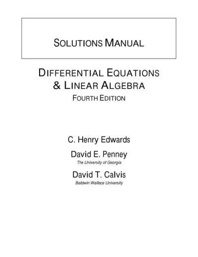 Textbook Guides
Solution Manual for Differential Equations and Linear Algebra, 4th Edition
Mathematics
658 pagesMay 2025 Exam Guides
Test Bank for Precalculus, 6th Edition
Mathematics
1051 pages175downloadsFeb 2025 Textbook Guides
Solution Manual For Introduction To Management Science, 11th Edition
Mathematics
437 pages167downloadsFeb 2025 Textbook Guides
Solution Manual For Derivatives Markets, 3rd Edition
Mathematics
358 pages143downloadsFeb 2025 Textbook Guides
Solution Manual for Geometry, 1st Edition
Mathematics
446 pages141downloadsFeb 2025 Textbook Guides
Solution Manual for Beginning Algebra, 7th Edition
Mathematics
479 pages139downloadsFeb 2025
Study this document with CramX
Once it is in your library, every tool can work from it.