

Solution Manual For Fundamentals Of Differential Equations, 8th Edition
- Mathematics
- 905 pages
- Shared May 2025
Solve your textbook questions faster and more accurately with Solution Manual For Fundamentals Of Differential Equations, 8th Edition, a reliable guide for every chapter.
Preview 16 of 905 pages
See the first 16 pages exactly as they appear in the document.
Page 1 Read page 1 as text
Contents Notes to the Instructor 1 Supplements . . . . . . . . . . . . . . . . . . . . . . . . . . . . . . . . . . . . . 1 Computer Labs . . . . . . . . . . . . . . . . . . . . . . . . . . . . . . . . . . . 2 Group Projects . . . . . . . . . . . . . . . . . . . . . . . . . . . . . . . . . . . . 2 Technical Writing Exercises . . . . . . . . . . . . . . . . . . . . . . . . . . . . . 2 Student Presentations . . . . . . . . . . . . . . . . . . . . . . . . . . . . . . . . 3 Homework Assignments . . . . . . . . . . . . . . . . . . . . . . . . . . . . . . . 3 Syllabus Suggestions . . . . . . . . . . . . . . . . . . . . . . . . . . . . . . . . . 4 Numerical, Graphical, and Qualitative Methods . . . . . . . . . . . . . . . . . . 4 Engineering/Physics Applications . . . . . . . . . . . . . . . . . . . . . . . . . 6 Biology/Ecology Applications . . . . . . . . . . . . . . . . . . . . . . . . . . . . 8 Supplemental Group Projects 10 Detailed Solutions & Answers to Even-Numbered Problems 17 CHAPTER 1 Introduction 17 Exercises 1.1 Detailed Solutions . . . . . . . . . . . . . . . . . . . . . . . . . 17 Exercises 1.2 Detailed Solutions . . . . . . . . . . . . . . . . . . . . . . . . . 18 Exercises 1.3 Detailed Solutions . . . . . . . . . . . . . . . . . . . . . . . . . 23 Exercises 1.4 Detailed Solutions . . . . . . . . . . . . . . . . . . . . . . . . . 25 Tables . . . . . . . . . . . . . . . . . . . . . . . . . . . . . . . . . . . . . . . . 29 Figures . . . . . . . . . . . . . . . . . . . . . . . . . . . . . . . . . . . . . . . 30 CHAPTER 2 First Order Differential Equations 35 Exercises 2.2 Detailed Solutions . . . . . . . . . . . . . . . . . . . . . . . . . 35 Exercises 2.3 Detailed Solutions . . . . . . . . . . . . . . . . . . . . . . . . . 43 Exercises 2.4 Detailed Solutions . . . . . . . . . . . . . . . . . . . . . . . . . 51 Exercises 2.5 Detailed Solutions . . . . . . . . . . . . . . . . . . . . . . . . . 59 Exercises 2.6 Detailed Solutions . . . . . . . . . . . . . . . . . . . . . . . . . 65 Review Problems Answers . . . . . . . . . . . . . . . . . . . . . . . . . . . . 74 Tables . . . . . . . . . . . . . . . . . . . . . . . . . . . . . . . . . . . . . . . . 75 Figures . . . . . . . . . . . . . . . . . . . . . . . . . . . . . . . . . . . . . . . 76 © i
Page 2 Page 3 Read page 3 as text
CHAPTER 3 Mathematical Models and Numerical Methods Involving First Order Equations 77 Exercises 3.2 Detailed Solutions . . . . . . . . . . . . . . . . . . . . . . . . . 77 Exercises 3.3 Detailed Solutions . . . . . . . . . . . . . . . . . . . . . . . . . 85 Exercises 3.4 Detailed Solutions . . . . . . . . . . . . . . . . . . . . . . . . . 91 Exercises 3.5 Answers . . . . . . . . . . . . . . . . . . . . . . . . . . . . . . . 100 Exercises 3.6 Answers . . . . . . . . . . . . . . . . . . . . . . . . . . . . . . . 101 Exercises 3.7 Answers . . . . . . . . . . . . . . . . . . . . . . . . . . . . . . . 101 Tables . . . . . . . . . . . . . . . . . . . . . . . . . . . . . . . . . . . . . . . . 103 Figures . . . . . . . . . . . . . . . . . . . . . . . . . . . . . . . . . . . . . . . 104 CHAPTER 4 Linear Second Order Equations 105 Exercises 4.1 Detailed Solutions . . . . . . . . . . . . . . . . . . . . . . . . . 105 Exercises 4.2 Detailed Solutions . . . . . . . . . . . . . . . . . . . . . . . . . 107 Exercises 4.3 Detailed Solutions . . . . . . . . . . . . . . . . . . . . . . . . . 115 Exercises 4.4 Detailed Solutions . . . . . . . . . . . . . . . . . . . . . . . . . 123 Exercises 4.5 Detailed Solutions . . . . . . . . . . . . . . . . . . . . . . . . . 128 Exercises 4.6 Detailed Solutions . . . . . . . . . . . . . . . . . . . . . . . . . 140 Exercises 4.7 Detailed Solutions . . . . . . . . . . . . . . . . . . . . . . . . . 147 Exercises 4.8 Detailed Solutions . . . . . . . . . . . . . . . . . . . . . . . . . 161 Exercises 4.9 Detailed Solutions . . . . . . . . . . . . . . . . . . . . . . . . . 164 Exercises 4.10 Detailed Solutions . . . . . . . . . . . . . . . . . . . . . . . . . 171 Review Problems Answers . . . . . . . . . . . . . . . . . . . . . . . . . . . . 175 Figures . . . . . . . . . . . . . . . . . . . . . . . . . . . . . . . . . . . . . . . 177 CHAPTER 5 Introduction to Systems and Phase Plane Analysis 181 Exercises 5.2 Answers . . . . . . . . . . . . . . . . . . . . . . . . . . . . . . . 181 Exercises 5.3 Answers . . . . . . . . . . . . . . . . . . . . . . . . . . . . . . . 183 Exercises 5.4 Answers . . . . . . . . . . . . . . . . . . . . . . . . . . . . . . . 184 Exercises 5.5 Answers . . . . . . . . . . . . . . . . . . . . . . . . . . . . . . . 186 Exercises 5.6 Answers . . . . . . . . . . . . . . . . . . . . . . . . . . . . . . . 186 Exercises 5.7 Answers . . . . . . . . . . . . . . . . . . . . . . . . . . . . . . . 186 Exercises 5.8 Answers . . . . . . . . . . . . . . . . . . . . . . . . . . . . . . . 187 Review Problems Answers . . . . . . . . . . . . . . . . . . . . . . . . . . . . 188 Tables . . . . . . . . . . . . . . . . . . . . . . . . . . . . . . . . . . . . . . . . 189 Figures . . . . . . . . . . . . . . . . . . . . . . . . . . . . . . . . . . . . . . . 191 CHAPTER 6 Theory of Higher-Order Linear Differential Equations 197 Exercises 6.1 Answers . . . . . . . . . . . . . . . . . . . . . . . . . . . . . . . 197 Exercises 6.2 Answers . . . . . . . . . . . . . . . . . . . . . . . . . . . . . . . 198 Exercises 6.3 Answers . . . . . . . . . . . . . . . . . . . . . . . . . . . . . . . 198 Exercises 6.4 Answers . . . . . . . . . . . . . . . . . . . . . . . . . . . . . . . 199 ii ©
Page 4 Read page 4 as text
Review Problems Answers . . . . . . . . . . . . . . . . . . . . . . . . . . . . 200 CHAPTER 7 Laplace Transforms 201 Exercises 7.2 Detailed Solutions . . . . . . . . . . . . . . . . . . . . . . . . . 201 Exercises 7.3 Detailed Solutions . . . . . . . . . . . . . . . . . . . . . . . . . 205 Exercises 7.4 Detailed Solutions . . . . . . . . . . . . . . . . . . . . . . . . . 211 Exercises 7.5 Detailed Solutions . . . . . . . . . . . . . . . . . . . . . . . . . 219 Exercises 7.6 Detailed Solutions . . . . . . . . . . . . . . . . . . . . . . . . . 228 Exercises 7.7 Detailed Solutions . . . . . . . . . . . . . . . . . . . . . . . . . 242 Exercises 7.8 Detailed Solutions . . . . . . . . . . . . . . . . . . . . . . . . . 250 Exercises 7.9 Detailed Solutions . . . . . . . . . . . . . . . . . . . . . . . . . 255 Review Problems Answers . . . . . . . . . . . . . . . . . . . . . . . . . . . . 265 Figures . . . . . . . . . . . . . . . . . . . . . . . . . . . . . . . . . . . . . . . 266 CHAPTER 8 Series Solutions of Differential Equations 271 Exercises 8.1 Answers . . . . . . . . . . . . . . . . . . . . . . . . . . . . . . . 271 Exercises 8.2 Answers . . . . . . . . . . . . . . . . . . . . . . . . . . . . . . . 272 Exercises 8.3 Answers . . . . . . . . . . . . . . . . . . . . . . . . . . . . . . . 273 Exercises 8.4 Answers . . . . . . . . . . . . . . . . . . . . . . . . . . . . . . . 274 Exercises 8.5 Answers . . . . . . . . . . . . . . . . . . . . . . . . . . . . . . . 275 Exercises 8.6 Answers . . . . . . . . . . . . . . . . . . . . . . . . . . . . . . . 275 Exercises 8.7 Answers . . . . . . . . . . . . . . . . . . . . . . . . . . . . . . . 277 Exercises 8.8 Answers . . . . . . . . . . . . . . . . . . . . . . . . . . . . . . . 278 Review Problems Answers . . . . . . . . . . . . . . . . . . . . . . . . . . . . 279 Figures . . . . . . . . . . . . . . . . . . . . . . . . . . . . . . . . . . . . . . . 280 CHAPTER 9 Matrix Methods for Linear Systems 281 Exercises 9.1 Answers . . . . . . . . . . . . . . . . . . . . . . . . . . . . . . . 281 Exercises 9.2 Answers . . . . . . . . . . . . . . . . . . . . . . . . . . . . . . . 281 Exercises 9.3 Answers . . . . . . . . . . . . . . . . . . . . . . . . . . . . . . . 282 Exercises 9.4 Answers . . . . . . . . . . . . . . . . . . . . . . . . . . . . . . . 285 Exercises 9.5 Answers . . . . . . . . . . . . . . . . . . . . . . . . . . . . . . . 287 Exercises 9.6 Answers . . . . . . . . . . . . . . . . . . . . . . . . . . . . . . . 289 Exercises 9.7 Answers . . . . . . . . . . . . . . . . . . . . . . . . . . . . . . . 290 Exercises 9.8 Answers . . . . . . . . . . . . . . . . . . . . . . . . . . . . . . . 292 Review Problems Answers . . . . . . . . . . . . . . . . . . . . . . . . . . . . 293 Figures . . . . . . . . . . . . . . . . . . . . . . . . . . . . . . . . . . . . . . . 295 CHAPTER 10 Partial Differential Equations 297 Exercises 10.2 Answers . . . . . . . . . . . . . . . . . . . . . . . . . . . . . . 297 Exercises 10.3 Answers . . . . . . . . . . . . . . . . . . . . . . . . . . . . . . 297 Exercises 10.4 Answers . . . . . . . . . . . . . . . . . . . . . . . . . . . . . . 298 © iii
Page 5 Read page 5 as text
Exercises 10.5 Answers . . . . . . . . . . . . . . . . . . . . . . . . . . . . . . 299 Exercises 10.6 Answers . . . . . . . . . . . . . . . . . . . . . . . . . . . . . . 300 Exercises 10.7 Answers . . . . . . . . . . . . . . . . . . . . . . . . . . . . . . 301 CHAPTER 11 Eigenvalue Problems and Sturm-Liouville Equations 303 Exercises 11.2 Answers . . . . . . . . . . . . . . . . . . . . . . . . . . . . . . 303 Exercises 11.3 Answers . . . . . . . . . . . . . . . . . . . . . . . . . . . . . . 304 Exercises 11.4 Answers . . . . . . . . . . . . . . . . . . . . . . . . . . . . . . 304 Exercises 11.5 Answers . . . . . . . . . . . . . . . . . . . . . . . . . . . . . . 305 Exercises 11.6 Answers . . . . . . . . . . . . . . . . . . . . . . . . . . . . . . 306 Exercises 11.7 Answers . . . . . . . . . . . . . . . . . . . . . . . . . . . . . . 308 Exercises 11.8 Answers . . . . . . . . . . . . . . . . . . . . . . . . . . . . . . 309 Review Problems Answers . . . . . . . . . . . . . . . . . . . . . . . . . . . . 309 CHAPTER 12 Stability of Autonomous Systems 311 Exercises 12.2 Answers . . . . . . . . . . . . . . . . . . . . . . . . . . . . . . 311 Exercises 12.3 Answers . . . . . . . . . . . . . . . . . . . . . . . . . . . . . . 311 Exercises 12.4 Answers . . . . . . . . . . . . . . . . . . . . . . . . . . . . . . 312 Exercises 12.5 Answers . . . . . . . . . . . . . . . . . . . . . . . . . . . . . . 312 Exercises 12.6 Answers . . . . . . . . . . . . . . . . . . . . . . . . . . . . . . 313 Exercises 12.7 Answers . . . . . . . . . . . . . . . . . . . . . . . . . . . . . . 313 Review Problems Answers . . . . . . . . . . . . . . . . . . . . . . . . . . . . 314 Figures . . . . . . . . . . . . . . . . . . . . . . . . . . . . . . . . . . . . . . . 315 CHAPTER 13 Existence and Uniqueness Theory 323 Exercises 13.1 Answers . . . . . . . . . . . . . . . . . . . . . . . . . . . . . . 323 Exercises 13.2 Answers . . . . . . . . . . . . . . . . . . . . . . . . . . . . . . 323 Exercises 13.3 Answers . . . . . . . . . . . . . . . . . . . . . . . . . . . . . . 324 Exercises 13.4 Answers . . . . . . . . . . . . . . . . . . . . . . . . . . . . . . 324 Review Problems Answers . . . . . . . . . . . . . . . . . . . . . . . . . . . . 324 Appendix A: Review of Integration Techniques 325 Exercises A Detailed Solutions . . . . . . . . . . . . . . . . . . . . . . . . . . 325 iv ©
Page 6 Read page 6 as text
Notes to the Instructor One goal in our writing has been to create flexible texts that afford the instructor a variety of topics and make available to the student an abundance of practice problems and projects. We recommend that the instructor read the discussion given in the preface in order to gain an overview of the prerequisites, topics of emphasis, and general philosophy of the text. Supplements Student’s Solutions Manual: By Viktor Maymeskul. Contains complete, worked-out solu- tions to most odd-numbered exercises, providing students with an excellent study tool. ISBN 13: 978-0-321-74834-8; ISBN 10: 0-321-74834-4. Companion Web site: Provides additional resources for both instructors and students, including helpful links keyed to sections of the text, access to Interactive Differential Equations, suggestions for incorporating Interactive Differential Equations modules, suggested syllabi, index of applications, and study tips for students. Access: www.pearsonhighered.com/nagle Interactive Differential Equations: By Beverly West (Cornell University), Steven Strogatz (Cornell University), Jean Marie McDill (California Polytechnic State University – San Luis Obispo), John Cantwell (St. Louis University), and Hubert Hohn (Massachusetts College of Arts) is a popular software directly tied to the text that focuses on helping students visualize concepts. Applications are drawn from engineering, physics, chemistry, and biology. Access: www.pearsonhighered.com/nagle Instructor’s MAPLE/MATHLAB/MATHEMATICA manuals: By Thomas W. Po- laski (Winthrop University), Bruno Welfert (Arizona State University), and Maurino Bautista (Rochester Institute of Technology). A collection of worksheets and projects to aid instructors in integrating computer algebra systems into their courses. Available in the Pearson Instructor Resource Center at www.pearsonhighered.com/irc . MATLAB Manual ISBN 13: 978-0-321-53015-8; ISBN 10: 0-321-53015-2 MAPLE Manual ISBN 13: 978-0-321-38842-1; ISBN 10: 0-321-38842-9 MATHEMATICA Manual ISBN 13: 978-0-321-52178-1; ISBN 10: 0-321-52178-1 © 1
Page 7 Read page 7 as text
Computer Labs A computer lab in connection with a differential equations course can add a whole new di- mension to the teaching and learning of differential equations. As more and more colleges and universities set up computer labs with software such as MAPLE, MATLAB, DERIVE, MATHEMATICA, PHASEPLANE, and MACMATH, there will be more opportunities to in- clude a lab as part of the differential equations course. In our teaching and in our texts, we have tried to provide a variety of exercises, problems, and projects that encourage the student to use the computer to explore. Even one or two hours at a computer generating phase plane diagrams can provide the students with a feeling of how they will use technology together with the theory to investigate real world problems. Furthermore, our experience is that they thoroughly enjoy these activities. Of course, the software, provided free with the texts, is especially convenient for such labs. Group Projects Although the projects that appear at the end of the chapters in the text can be worked out by the conscientious student working alone, making them group projects adds a social element that encourages discussion and interactions that simulate a professional work place atmosphere. Group sizes of 3 or 4 seem to be optimal. Moreover, requiring that each individual student separately write up the group’s solution as a formal technical report for grading by the instructor also contributes to the professional flavor. Typically, our students each work on 3 or 4 projects per semester. If class time permits, oral presentations by the groups can be scheduled and help to improve the communication skills of the students. The role of the instructor is, of course, to help the students solve these elaborate problems on their own and to recommend additional reference material when appropriate. Some additional Group Projects are presented in this guide (see page 10). Technical Writing Exercises The technical writing exercises at the end of most chapters invite students to make documented responses to questions dealing with the concepts in the chapter. This not only gives students an opportunity to improve their writing skills, but it helps them organize their thoughts and better understand the new concepts. Moreover, many questions deal with critical thinking 2 ©
Page 8 Read page 8 as text
skills that will be useful in their careers as engineers, scientists, or mathematicians. Since most students have little experience with technical writing, it may be necessary to return ungraded the first few technical writing assignments with comments and have the students redo the the exercise. This has worked well in our classes and is much appreciated by the students. Handing out a “model” technical writing response is also helpful for the students. Student Presentations It is not uncommon for an instructor to have students go to the board and present a solution to a problem. Differential equations is so rich in theory and applications that it is an excellent course to allow (require) a student to give a presentation on a special application (e.g., almost any topic from Chapters 3 and 5), on a new technique not covered in class (e.g., material from Section 2.6, Projects A, B, or C in Chapter 4), or on additional theory (e.g., material from Chapter 6 which generalizes the results in Chapter 4). In addition to improving students’ communication skills, these “special” topics are long remembered by the students. Here, too, working in groups of 3 or 4 and sharing the presentation responsibilities can add substantially to the interest and quality of the presentation. Students should also be encouraged to enliven their communication by building physical models, preparing part of their lectures with the aid of video technology, and utilizing appropriate internet web sites. Homework Assignments We would like to share with you an obvious, non-original, but effective method to encourage students to do homework problems. An essential feature is that it requires little extra work on the part of the instructor or grader. We assign homework problems (about 5 of them) after each lecture. At the end of the week (Fridays), students are asked to turn in their homework (typically, 3 sets) for that week. We then choose at random one problem from each assignment (typically, a total of 3) that will be graded. (The point is that the student does not know in advance which problems will be chosen.) Full credit is given for any of the chosen problems for which there is evidence that the student has made an honest attempt at solving. The homework problem sets are returned to the students at the next meeting (Mondays) with grades like 0 / 3, 1 / 3, 2 / 3, or 3 / 3 indicating the proportion of problems for which the student received credit. The homework grades are tallied at the end of the semester and count as one test grade. Certainly, there are variations © 3
Page 9 Read page 9 as text
on this theme. The point is that students are motivated to do their homework. Syllabus Suggestions To serve as a guide in constructing a syllabus for a one-semester or two-semester course, the prefaces to the texts list sample outlines that emphasize methods, applications, theory, partial differential equations, phase plane analysis, computation, or combinations of these. As a further guide in making a choice of subject matter, we provide (starting on the next page) a listing of text material dealing with some common areas of emphasis. Numerical, Graphical, and Qualitative Methods The sections and projects dealing with numerical, graphical, and qualitative techniques of solving differential equations include: Section 1.3: Direction Fields Section 1.4: The Approximation Method of Euler Project A for Chapter 1: Taylor Series Method Project B for Chapter 1: Picard’s Method Project C for Chapter 1: The Phase Line Section 3.6: Improved Euler’s Method , which includes step-by-step outlines of the im- proved Euler’s method subroutine and improved Euler’s method with tolerance. These outlines are easy for the student to translate into a computer program (pp. 127–128). Section 3.7: Higher-Order Numerical Methods : Taylor and Runge-Kutta , which includes outlines for the Fourth Order Runge-Kutta subroutine and algorithm with tolerance (see pp. 135–136). Project H for Chapter 3: Stability of Numerical Methods Project I for Chapter 3: Period Doubling and Chaos 4 ©
Page 10 Read page 10 as text
Section 4.8: Qualitative Considerations for Variable Coefficient and Non-linear Equa- tions , which discusses the energy integral lemma, as well as the Airy, Bessel, Duffing, and van der Pol equations. Section 5.3: Solving Systems and Higher-Order Equations Numerically , which describes the vectorized forms of Euler’s method and the Fourth Order Runge-Kutta method, and discusses an application to population dynamics. Section 5.4: Introduction to the Phase Plane , which introduces the study of trajectories of autonomous systems, critical points, and stability. Section 5.8: Dynamical Systems, Poincar´ e Maps, and Chaos , which discusses the use of numerical methods to approximate the Poincar` e map and how to interpret the results. Project A for Chapter 6: Computer Algebra Systems and Exponential Shift Project D for Chapter 6: Higher-Order Difference Equations Project A for Chapter 8: Alphabetization Algorithms Project D for Chapter 10: Numerical Method for Δ u = f on a Rectangle Project D for Chapter 11: Shooting Method Project E for Chapter 11: Finite-Difference Method for Boundary Value Problems Project C for Chapter 12: Computing Phase Plane Diagrams Project D for Chapter 12: Ecosystem of Planet GLIA-2 Section 13.1: Introduction: Successive Approximations Appendix B: Newton’s Method Appendix C: Simpson’s Rule Appendix E: Method of Least Squares Appendix F: Runge-Kutta Procedure for Equations © 5
Page 11 Read page 11 as text
The instructor who wishes to emphasize numerical methods should also note that the text contains an extensive chapter of series solutions of differential equations (Chapter 8). Engineering/Physics Applications Since Laplace transforms is a subject vital to engineering, we have included a detailed chapter on this topic – see Chapter 7. Stability is also an important subject for engineers, so we have included an introduction to the subject in Section 5.4 along with an entire chapter addressing this topic – see Chapter 12. Further material dealing with engineering/physics applications include: Project C for Chapter 2: Torricelli’s Law of Fluid Flow . Project I for Chapter 2: Designing a Solar Collector . Section 3.1: Mathematical Modeling . Section 3.2: Compartmental Analysis , which contains a discussion of mixing problems and of population models. Section 3.3: Heating and Cooling off Buildings , which discusses temperature variations in the presence of air conditioning or furnace heating. Section 3.4: Newtonian Mechanics . Section 3.5: Electrical Circuits . Project C for Chapter 3: Curve of Pursuit . Project D for Chapter 3: Aircraft Guidance in a Crosswind . Project E for Chapter 3: Feedback and the Op Amp . Project F for Chapter 3: Bang-Bang Controls . Section 4.1: Introduction: The Mass-Spring Oscillator . Section 4.8: Qualitative Considerations for Variable-Coefficient and Non-linear Equa- tions . Section 4.9: A Closer Look at Free Mechanical Vibrations . 6 ©
Page 12 Read page 12 as text
Section 4.10: A Closer Look at Forced Mechanical Vibrations . Project B for Chapter 4: Apollo Re-entry Project C for Chapter 4: Simple Pendulum Section 5.1: Interconnected Fluid Tanks . Section 5.4: Introduction to the Phase PLane . Section 5.6: Coupled Mass-Spring Systems . Section 5.7: Electrical Systems . Section 5.8: Dynamical Systems, Poincar´ e Maps, and Chaos . Project A for Chapter 5: Designing a Landing System for Interplanetary Travel . Project C for Chapter 5: Things that Bob . Project D for Chapter 5: Hamiltonian Systems . Project C for Chapter 6: Transverse Vibrations of a Beam . Chapter 7: Laplace Transforms , which in addition to basic material includes discussions of transfer functions, the Dirac delta function, and frequency response modelling. Project B for Chapter 8, Spherically Symmetric Solutions to Schr¨ odinger’s Equation for the Hydrogen Atom Project D for Chapter 8, Buckling of a Tower Project E for Chapter 8, Aging Spring and Bessel Functions Section 9.6: Complex Eigenvalues , includes discussion of normal (natural) frequencies. Project B for Chapter 9: Matrix Laplace Transform Method . Project C for Chapter 9: Undamped Second-Order Systems . Chapter 10: Partial Differential Equations , which includes sections on Fourier series, the heat equation, wave equation, and Laplace’s equation. © 7
Page 13 Read page 13 as text
Project A for Chapter 10: Steady-State Temperature Distribution in a Circular Cylinder . Project B for Chapter 10: A Laplace Transform Solution of the Wave Equation . Project A for Chapter 11: Hermite Polynomials and the Harmonic Oscillator . Section 12.4: Energy Methods , which addresses both conservative and non-conservative autonomous mechanical systems. Project A for Chapter 12: Solitons and Korteweg-de Vries Equation . Project B for Chapter 12: Burger’s Equation . Students of engineering and physics would also find Chapter 8 on series solutions particularly useful, especially Section 8.8 on special functions. Biology/Ecology Applications Project C for Chapter 1: The Phase Plane , which discusses the logistic population model and bifurcation diagrams for population control. Project A for Chapter 2: Oil Spill in a Canal . Project B for Chapter 2: Differential Equations in Clinical Medicine . Section 3.1: Mathematical Modelling . Section 3.2: Compartmental Analysis , which contains a discussion of mixing problems and population models. Project A for Chapter 3: Dynamics of HIV Infection . Project B for Chapter 3: Aquaculture , which deals with a model of raising and harvesting catfish. Section 5.1: Interconnected Fluid Tanks , which introduces systems of equations. Section 5.3: Solving Systems and Higher-Order Equations Numerically , which contains an application to population dynamics. 8 ©
Page 14 Read page 14 as text
Section 5.5: Applications to Biomathematics: Epidemic and Tumor Growth Models . Project B for Chapter 5: Spread of Staph Infections in Hospitals – Part I . Project E for Chapter 5: Cleaning Up the Great Lakes Project F for Chapter 5: A Growth Model for Phytoplankton – Part I . Problem 19 in Exercises 10.5 , which involves chemical diffusion through a thin layer. Project D for Chapter 12: Ecosystem on Planet GLIA-2 Project E for Chapter 12: Spread of Staph Infections in Hospitals – Part II . Project F for Chapter 12: A Growth Model for Phytoplankton – Part II . The basic content of the remainder of this instructor’s manual consists of supplemental group projects, answers to the even-numbered problems, and detailed solutions to the most even- numbered problems in Chapters 1, 2, 3, 4, and 7. These answers are not available any place else since the text and the Student’s Solutions Manual only provide answers and solutions to odd-numbered problems. We would appreciate any comments you may have concerning the answers in this manual. These comments can be sent to the authors’ email addresses below. We also would encourage sharing with us (the authors and users of the texts) any of your favorite group projects. E. B. Saff A. D. Snider Edward.B.Saff@Vanderbilt.edu snider@eng.usf.edu © 9
Page 15 Read page 15 as text
Group Projects for Chapter 3 Delay Differential Equations In our discussion of mixing problems in Section 3.2, we encountered the initial value problem x ′ ( t ) = 6 − 3 500 x ( t − t 0 ) , (0.1) x ( t ) = 0 for x ∈ [ − t 0 , 0] , where t 0 is a positive constant. The equation in (0.1) is an example of a delay differ- ential equation . These equations differ from the usual differential equations by the presence of the shift ( t − t 0 ) in the argument of the unknown function x ( t ). In general, these equations are more difficult to work with than are regular differential equations, but quite a bit is known about them. 1 (a) Show that the simple linear delay differential equation x ′ = ax ( t − b ) , (0.2) where a , b are constants, has a solution of the form x ( t ) = Ce st for any constant C , provided s satisfies the transcendental equation s = ae − bs . (b) A solution to (0.2) for t > 0 can also be found using the method of steps . Assume that x ( t ) = f ( t ) for − b ≤ t ≤ 0. For 0 ≤ t ≤ b , equation (0.2) becomes x ′ ( t ) = ax ( t − b ) = af ( t − b ) , and so x ( t ) = t ∫ 0 af ( ν − b ) dν + x (0) . Now that we know x ( t ) on [0 , b ], we can repeat this procedure to obtain x ( t ) = t ∫ b ax ( ν − b ) dν + x ( b ) for b ≤ x ≤ 2 b . This process can be continued indefinitely. 1 See, for example, Differential–Difference Equations , by R. Bellman and K. L. Cooke, Academic Press, New York, 1963, or Ordinary and Delay Differential Equations , by R. D. Driver, Springer–Verlag, New York, 1977 10 ©
Page 16 Read page 16 as text
Use the method of steps to show that the solution to the initial value problem x ′ ( t ) = − x ( t − 1) , x ( t ) = 1 on [ − 1 , 0] , is given by x ( t ) = n ∑ k =0 ( − 1) k [ t − ( k − 1)] k k ! , for n − 1 ≤ t ≤ n , where n is a nonnegative integer. (This problem can also be solved using the Laplace transform method of Chapter 7.) (c) Use the method of steps to compute the solution to the initial value problem given in (0.1) on the interval 0 ≤ t ≤ 15 for t 0 = 3. Extrapolation When precise information about the form of the error in an approximation is known, a technique called extrapolation can be used to improve the rate of convergence. Suppose the approximation method converges with rate O ( h p ) as h → 0 (cf. Section 3.6). From theoretical considerations, assume we know, more precisely, that y ( x ; h ) = φ ( x ) + h p a p ( x ) + O ( h p +1 ) , (0.3) where y ( x ; h ) is the approximation to φ ( x ) using step size h and a p ( x ) is some function that is independent of h (typically, we do not know a formula for a p ( x ), only that it exists). Our goal is to obtain approximations that converge at the faster rate than O ( h p +1 ). We start by replacing h by h/ 2 in (0.3) to get y ( x ; h 2 ) = φ ( x ) + h p 2 p a p ( x ) + O ( h p +1 ) . If we multiply both sides by 2 p and subtract equation (0.3), we find 2 p y ( x ; h 2 ) − y ( x ; h ) = (2 p − 1) φ ( x ) + O ( h p +1 ) . Solving for φ ( x ) yields φ ( x ) = 2 p y ( x ; h/ 2) − y ( x ; h ) 2 p − 1 + O ( h p +1 ) . © 11
889 more pages in the full document
Unlock it once and it stays in your library, ready to chat with or turn into flashcards.
Unlock the full documentMore Mathematics study materials
See all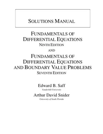 Textbook Guides
Solution Manual for Fundamentals of Differential Equations, 9th Edition
Mathematics
344 pagesMay 2025 Exam Guides
Test Bank for Precalculus, 6th Edition
Mathematics
1051 pages175downloadsFeb 2025 Textbook Guides
Solution Manual For Introduction To Management Science, 11th Edition
Mathematics
437 pages167downloadsFeb 2025 Textbook Guides
Solution Manual For Derivatives Markets, 3rd Edition
Mathematics
358 pages143downloadsFeb 2025 Textbook Guides
Solution Manual for Geometry, 1st Edition
Mathematics
446 pages141downloadsFeb 2025 Textbook Guides
Solution Manual for Beginning Algebra, 7th Edition
Mathematics
479 pages139downloadsFeb 2025 Textbook Guides
Solution Manual for Developmental Mathematics, 1st Edition
Mathematics
1623 pages137downloadsFeb 2025 Textbook Guides
Solution Manual for Elementary and Intermediate Algebra: Graphs and Models, 5th Edition
Mathematics
1278 pages126downloadsFeb 2025
Study this document with CramX
Once it is in your library, every tool can work from it.