

Solution Manual For Fundamentals of Heat and Mass Transfer, 8th Edition
- Mechanical Engineering
- 1985 pages
- Shared May 2025
Solution Manual For Fundamentals of Heat and Mass Transfer, 8th Edition is your textbook problem-solver, offering clear and concise solutions to difficult questions.
Preview 16 of 1985 pages
See the first 16 pages exactly as they appear in the document.
Page 1 Read page 1 as text
PROBLEM 1.1 KNOWN: Temperature distribution in wall of Example 1.1. FIND: Heat fluxes and heat rates at x = 0 and x = L . SCHEMATIC: ASSUMPTIONS: (1) One-dimensional conduction through the wall, (2) constant thermal conductivity, (3) no internal thermal energy generation within the wall. PROPERTIES: Thermal conductivity of wall (given): k = 1.7 W/m·K. ANALYSIS: The heat flux in the wall is by conduction and is described by Fourier’s law, x dT q k dx ′′ = − (1) Since the temperature distribution is T ( x ) = a + bx , the temperature gradient is dT b dx = (2) Hence, the heat flux is constant throughout the wall, and is ( ) 2 1.7 W/m K 1000 K/m 1700 W/m x dT q k kb dx ′′ = − = − = − ⋅ × − = < Since the cross-sectional area through which heat is conducted is constant, the heat rate is constant and is ( ) 2 ( ) 1700 W/m 1.2 m × 0.5 m 1020 W x x q q W H ′′ = × × = × = < Because the heat rate into the wall is equal to the heat rate out of the wall, steady-state conditions exist. < COMMENTS: (1) If the heat rates were not equal, the internal energy of the wall would be changing with time. (2) The temperatures of the wall surfaces are T 1 = 1400 K and T 2 = 1250 K.
Page 2 Page 3 Read page 3 as text
PROBLEM 1.2 KNOWN: Thermal conductivity, thickness and temperature difference across a sheet of rigid extruded insulation. FIND: (a) The heat flux through a 3 m × 3 m sheet of the insulation, (b) the heat rate through the sheet, and (c) the thermal conduction resistance of the sheet. SCHEMATIC: ASSUMPTIONS: (1) One-dimensional conduction in the x-direction, (2) Steady-state conditions, (3) Constant properties. ANALYSIS: (a) From Equation 1.2 the heat flux is 1 2 x 2 T - T dT W 12 K W q = -k = k = 0.029 × = 13.9 dx L m K 0.025 m m ′′ ⋅ < (b) The heat rate is 2 x x 2 W q = q A = 13.9 × 9 m = 125 W m ′′ ⋅ < (c) From Eq. 1.11, the thermal resistance is t,cond x R T / q = 12 K /125 W 0.096 K/W = ∆ = < COMMENTS: (1) Be sure to keep in mind the important distinction between the heat flux (W/m 2 ) and the heat rate (W). (2) The direction of heat flow is from hot to cold. (3) Note that a temperature difference may be expressed in kelvins or degrees Celsius. (4) The conduction thermal resistance for a plane wall could equivalently be calculated from R t,cond = L/kA. q cond A = 4 m 2 T 2 T 1 k = 0.029 x L = 20 mm T 1 – T 2 = 10 ˚ C q cond A = 4 m 2 T 2 T 1 k = 0.029 x L = 20 mm T 1 – T 2 = 10 ˚ C 9 m 2 12 ° C 25 mm q cond A = 4 m 2 T 2 T 1 k = 0.029 x L = 20 mm T 1 – T 2 = 10 ˚ C q cond A = 4 m 2 T 2 T 1 k = 0.029 x L = 20 mm T 1 – T 2 = 10 ˚ C 9 m 2 12 ° C 25 mm
Page 4 Read page 4 as text
PROBLEM 1.3 KNOWN: Thickness and thermal conductivity of a wall. Heat flux applied to one face and temperatures of both surfaces. FIND: Whether steady-state conditions exist. SCHEMATIC : ASSUMPTIONS : (1) One-dimensional conduction, (2) Constant properties, (3) No internal energy generation. ANALYSIS: Under steady-state conditions an energy balance on the control volume shown is 2 in out cond 1 2 ( ) / 12 W/m K(50 C 30 C) / 0.01 m 24,000 W/m q q q k T T L ′′ ′′ ′′ = = = − = ⋅ ° − ° = Since the heat flux in at the left face is only 20 W/m 2 , the conditions are not steady state. < COMMENTS: If the same heat flux is maintained until steady-state conditions are reached, the steady-state temperature difference across the wall will be ∆ T = 2 / 20 W/m 0.01 m /12 W/m K 0.0167 K q L k ′′ = × ⋅ = which is much smaller than the specified temperature difference of 20 ° C. q ” = 20 W/m 2 L = 10 mm k = 12 W/m ∙ K T 1 = 50 ° C T 2 = 30 ° C q ″ cond
Page 5 Read page 5 as text
PROBLEM 1.4 KNOWN: Inner surface temperature and thermal conductivity of a concrete wall. FIND: Heat loss by conduction through the wall as a function of outer surface temperatures ranging from -15 to 38 ° C. SCHEMATIC: ASSUMPTIONS: (1) One-dimensional conduction in the x-direction, (2) Steady-state conditions, (3) Constant properties. ANALYSIS: From Fourier’s law, if x q ′′ and k are each constant it is evident that the gradient, x dT dx q k ′′ = − , is a constant, and hence the temperature distribution is linear. The heat flux must be constant under one-dimensional, steady-state conditions; and k is approximately constant if it depends only weakly on temperature. The heat flux and heat rate when the outside wall temperature is T 2 = -15 ° C are ( ) 2 1 2 x 25 C 15 C dT T T q k k 1W m K 133.3 W m dx L 0.30 m − − − ′′ = − = = ⋅ = . (1) 2 2 x x q q A 133.3 W m 20 m 2667 W ′′ = × = × = . (2) < Combining Eqs. (1) and (2), the heat rate q x can be determined for the range of outer surface temperature, -15 ≤ T 2 ≤ 38 ° C, with different wall thermal conductivities, k. For the concrete wall, k = 1 W/m ⋅ K, the heat loss varies linearly from +2667 W to -867 W and is zero when the inside and outer surface temperatures are the same. The magnitude of the heat rate increases with increasing thermal conductivity. COMMENTS: Without steady-state conditions and constant k, the temperature distribution in a plane wall would not be linear. -20 -10 0 10 20 30 40 Ambient air temperature, T2 (C) -1500 -500 500 1500 2500 3500 Heat loss, qx (W) Wall thermal conductivity, k = 1.25 W/m.K k = 1 W/m.K, concrete wall k = 0.75 W/m.K Outside surface -20 -10 0 10 20 30 40 Ambient air temperature, T2 (C) -1500 -500 500 1500 2500 3500 Heat loss, qx (W) Wall thermal conductivity, k = 1.25 W/m.K k = 1 W/m.K, concrete wall k = 0.75 W/m.K Outside surface
Page 6 Read page 6 as text
PROBLEM 1.5 KNOWN: Dimensions, thermal conductivity and surface temperatures of a concrete slab. Efficiency of gas furnace and cost of natural gas. FIND: Daily cost of heat loss. SCHEMATIC: Furnace, = 0.90 η f Natural gas, C = $0.01/MJ g Concrete, k = 1.4 W/m-K t = 0.2 m L = 11 m W = 8 m T = 17 C 1 o T = 10 C 2 o q Warm air ASSUMPTIONS: (1) Steady state, (2) One-dimensional conduction, (3) Constant properties. ANALYSIS: The rate of heat loss by conduction through the slab is ( ) ( ) 1 2 T T 7 C q k LW 1.4 W / m K 11m 8 m 4312 W t 0.20 m − ° = = ⋅ × = < The daily cost of natural gas that must be combusted to compensate for the heat loss is ( ) ( ) g d 6 f q C 4312 W $0.02 / MJ C t 24 h / d 3600s / h $8.28 / d 0.9 10 J / MJ η × = ∆ = × = × < COMMENTS: The loss could be reduced by installing a floor covering with a layer of insulation between it and the concrete.
Page 7 Read page 7 as text
PROBLEM 1.6 KNOWN: Heat flux and surface temperatures associated with a wood slab of prescribed thickness. FIND: Thermal conductivity, k, of the wood. SCHEMATIC: ASSUMPTIONS: (1) One-dimensional conduction in the x-direction, (2) Steady-state conditions, (3) Constant properties. ANALYSIS: Subject to the foregoing assumptions, the thermal conductivity may be determined from Fourier’s law, Eq. 1.2. Rearranging, ( ) L W 0.05m k=q 40 T T m 40-20 C x 2 1 2 ′′ = - k = 0.10 W / m K. ⋅ < COMMENTS: Note that the ° C or K temperature units may be used interchangeably when evaluating a temperature difference.
Page 8 Read page 8 as text
PROBLEM 1.7 KNOWN: Inner and outer surface temperatures and thermal resistance of a glass window of prescribed dimensions. FIND: Heat loss through window. Thermal conductivity of glass. SCHEMATIC: A = 1m x 3m = 3m 2 , R t,cond = 1.19 x 10 -3 K/W ASSUMPTIONS: (1) One-dimensional conduction in the x-direction, (2) Steady-state conditions, (3) Constant properties. ANALYSIS: From Eq. 1.11, ( ) 3 t,cond 15-5 C T T q 8400 W R 1.19 10 K/W 1 2 x - - = = = × < The thermal resistance due to conduction for a plane wall is related to the thermal conductivity and dimensions according to t,cond R = L/kA Therefore 3 2 t,cond k L/(R A) 0.005 m / (1.19 10 K/W 3 m ) 1.40 W/m K - = = × × = ⋅ < COMMENTS: The thermal conductivity value agrees with the value for glass in Table A.3.
Page 9 Read page 9 as text
PROBLEM 1.8 KNOWN: Net power output, average compressor and turbine temperatures, shaft dimensions and thermal conductivity. FIND: (a) Comparison of the conduction rate through the shaft to the predicted net power output of the device, (b) Plot of the ratio of the shaft conduction heat rate to the anticipated net power output of the device over the range 0.005 m ≤ L ≤ 1 m and feasibility of a L = 0.005 m device. SCHEMATIC : ASSUMPTIONS : (1) Steady-state conditions, (2) Constant properties, (3) Net power output is proportional to the volume of the gas turbine. PROPERTIES: Shaft (given): k = 40 W/m ⋅ K. ANALYSIS: (a) The conduction through the shaft may be evaluated using Fourier’s law, yielding ( ) ( ) 2 3 2 ( ) 40W/m K(1000 400) C " / 4 (70 10 m) / 4 92.4W 1m h c c k T T q q A d L π π − − ⋅ − ° = = = × = The ratio of the conduction heat rate to the net power output is 6 6 92.4W 18.5 10 5 10 W q r P − = = = × × < (b) The volume of the turbine is proportional to L 3 . Designating L a = 1 m, d a = 70 mm and P a as the shaft length, shaft diameter, and net power output, respectively, in part (a), d = d a × ( L/L a ); P = P a × ( L/L a ) 3 and the ratio of the conduction heat rate to the net power output is ( ) ( ) ( ) 2 2 2 3 2 3 2 6 6 2 2 2 ( ) ( ) ( ) / 4 / / 4 / " 4 ( / ) 40W/m K(1000 400) C (70 10 m) 1m / 5 10 W 18.5 10 m 4 = h c h c h c a a a a a c a a k T T k T T k T T d d L L d L P q A L L r P P P L L L L L π π π π − − − − − = = = = ⋅ − ° × × × × = Continued… L = 1m d = 70 mm P = 5 MW Turbine Compressor Shaft T h = 1000 ° C T c = 400 ° C Combustion chamber L = 1m d = 70 mm P = 5 MW Turbine Compressor Shaft T h = 1000 ° C T c = 400 ° C Combustion chamber k = 40 W/m ∙ K
Page 10 Read page 10 as text
PROBLEM 1.8 (Cont.) The ratio of the shaft conduction to net power is shown below. At L = 0.005 m = 5 mm, the shaft conduction to net power output ratio is 0.74. The concept of the very small turbine is not feasible since it will be unlikely that the large temperature difference between the compressor and turbine can be maintained. < COMMENTS: (1) The thermodynamics analysis does not account for heat transfer effects and is therefore meaningful only when heat transfer can be safely ignored, as is the case for the shaft in part (a). (2) Successful miniaturization of thermal devices is often hindered by heat transfer effects that must be overcome with innovative design. Ratio of shaft conduction to net power 0 0.2 0.4 0.6 0.8 1 L (m) 0.0001 0.001 0.01 0.1 1 r
Page 11 Read page 11 as text
PROBLEM 1.9 KNOWN: Heat flux at one face and air temperature and convection coefficient at other face of plane wall. Temperature of surface exposed to convection. FIND: If steady-state conditions exist. If not, whether the temperature is increasing or decreasing. SCHEMATIC : ASSUMPTIONS : (1) One-dimensional conduction, (2) No internal energy generation. ANALYSIS: Conservation of energy for a control volume around the wall gives st in out g dE E E E dt = − + [ ] st in in 2 2 2 ( ) ( ) 20 W/m 20 W/m K(50 C 30 C) 380 W/m s s dE q A hA T T q h T T A dt A A ∞ ∞ ′′ ′′ = − − = − − = − ⋅ ° − ° = − Since dE st / dt ≠ 0, the system is not at steady-state. < Since dE st / dt < 0, the stored energy is decreasing, therefore the wall temperature is decreasing. < COMMENTS: When the surface temperature of the face exposed to convection cools to 31 ° C, q in = q out and dE st / dt = 0 and the wall will have reached steady-state conditions. q ” = 20 W/m 2 T s = 50 ° C h = 20 W/m 2 ∙ K T ∞ = 30 ° C Air q ” conv
Page 12 Read page 12 as text
PROBLEM 1.10 KNOWN: Expression for variable thermal conductivity of a wall. Constant heat flux. Temperature at x = 0. FIND: Expression for temperature gradient and temperature distribution. SCHEMATIC: ASSUMPTIONS: (1) One-dimensional conduction. ANALYSIS: The heat flux is given by Fourier’s law, and is known to be constant, therefore x dT q k constant dx ′′ = − = Solving for the temperature gradient and substituting the expression for k yields x x q q dT dx k ax b ′′ ′′ = − = − + < This expression can be integrated to find the temperature distribution, as follows: x q dT dx dx dx ax b ′′ = − + ∫ ∫ Since x q constant ′′ = , we can integrate the right hand side to find ( ) x q T ln ax b c a ′′ = − + + where c is a constant of integration. Applying the known condition that T = T 1 at x = 0, we can solve for c. Continued… q ” x k = a x + b T 1
Page 13 Read page 13 as text
PROBLEM 1.10 (Cont.) 1 x 1 x 1 T(x 0) T q ln b c T a q c T ln b a = = ′′ − + = ′′ = + Therefore, the temperature distribution is given by ( ) x x 1 q q T ln ax b T ln b a a ′′ ′′ = − + + + < x 1 q b T ln a ax b ′′ = + + < COMMENTS: Temperature distributions are not linear in many situations, such as when the thermal conductivity varies spatially or is a function of temperature. Non-linear temperature distributions may also evolve if internal energy generation occurs or non-steady conditions exist.
Page 14 Read page 14 as text
PROBLEM 1.11 KNOWN: Thickness, diameter and inner surface temperature of bottom of pan used to boil water. Rate of heat transfer to the pan. FIND: Outer surface temperature of pan for an aluminum and a copper bottom. SCHEMATIC: ASSUMPTIONS: (1) One-dimensional, steady-state conduction through bottom of pan. ANALYSIS: From Fourier’s law, the rate of heat transfer by conduction through the bottom of the pan is T T 1 2 q kA L − = Hence, qL T T 1 2 kA = + where ( ) 2 2 2 A D / 4 0.22m / 4 0.038 m . π π = = = Aluminum : ( ) ( ) 600W 0.008 m T 110 C 110.5 C 1 2 240 W/m K 0.038 m = + = ⋅ < Copper : ( ) ( ) 600W 0.008 m T 110 C 110.3 C 1 2 390 W/m K 0.038 m = + = ⋅ < COMMENTS: Although the temperature drop across the bottom is slightly larger for aluminum (due to its smaller thermal conductivity), it is sufficiently small to be negligible for both materials. To a good approximation, the bottom may be considered isothermal at T ≈ 110 ° C, which is a desirable feature of pots and pans. Aluminum (k=240 W/m-K) or Copper (k=390 W/m-K) L = 5 mm D = 200 mm q = 600 W T 1 T = 110 C 2 o L = 8 mm D = 220 mm
Page 15 Read page 15 as text
PROBLEM 1.12 KNOWN: Hand experiencing convection heat transfer with moving air and water. FIND: Determine which condition feels colder. Contrast these results with a heat loss of 30 W/m 2 under normal room conditions. SCHEMATIC: ASSUMPTIONS: (1) Temperature is uniform over the hand’s surface, (2) Convection coefficient is uniform over the hand, and (3) Negligible radiation exchange between hand and surroundings in the case of air flow. ANALYSIS: The hand will feel colder for the condition which results in the larger heat loss. The heat loss can be determined from Newton’s law of cooling, Eq. 1.3a, written as ( ) s q h T T ∞ ′′ = − For the air stream: ( ) 2 2 air q 40 W m K 30 8 K 1,520 W m ′′ = ⋅ − − = < For the water stream: ( ) 2 2 water q 900 W m K 30 10 K 18, 000 W m ′′ = ⋅ − = < COMMENTS: The heat loss for the hand in the water stream is an order of magnitude larger than when in the air stream for the given temperature and convection coefficient conditions. In contrast, the heat loss in a normal room environment is only 30 W/m 2 which is a factor of 50 times less than the loss in the air stream. In the room environment, the hand would feel comfortable; in the air and water streams, as you probably know from experience, the hand would feel uncomfortably cold since the heat loss is excessively high.
Page 16 Read page 16 as text
PROBLEM 1.13 KNOWN: Power required to maintain the surface temperature of a long, 25-mm diameter cylinder with an imbedded electrical heater for different air velocities. FIND: (a) Determine the convection coefficient for each of the air velocity conditions and display the results graphically, and (b) Assuming that the convection coefficient depends upon air velocity as h = CV n , determine the parameters C and n. SCHEMATIC: V(m/s) 1 2 4 8 12 ¢ P e (W/m) 450 658 983 1507 1963 h (W/m 2 ⋅ K) 22.0 32.2 48.1 73.8 96.1 ASSUMPTIONS: (1) Temperature is uniform over the cylinder surface, (2) Negligible radiation exchange between the cylinder surface and the surroundings, (3) Steady-state conditions. ANALYSIS: (a) From an overall energy balance on the cylinder, the power dissipated by the electrical heater is transferred by convection to the air stream. Using Newton’s law of cooling on a per unit length basis, ( )( ) e s P h D T T π ∞ ′ = − where e P ′ is the electrical power dissipated per unit length of the cylinder. For the V = 1 m/s condition, using the data from the table above, find ( ) 2 h 450 W m 0.025 m 300 40 C 22.0 W m K π = × − = ⋅ < Repeating the calculations, find the convection coefficients for the remaining conditions which are tabulated above and plotted below. Note that h is not linear with respect to the air velocity. (b) To determine the (C,n) parameters, we plotted h vs. V on log-log coordinates. Choosing C = 22.12 W/m 2 ⋅ K(s/m) n , assuring a match at V = 1, we can readily find the exponent n from the slope of the h vs. V curve. From the trials with n = 0.8, 0.6 and 0.5, we recognize that n = 0.6 is a reasonable choice. Hence, C = 22.12 and n = 0.6. < 0 2 4 6 8 10 12 Air velocity, V (m/s) 20 40 60 80 100 Coefficient, h (W/m^2.K) Data, smooth curve, 5-points 1 2 4 6 8 10 Air velocity, V (m/s) 10 20 40 60 80 100 Coefficient, h (W/m^2.K) Data , smooth curve, 5 points h = C * V^n, C = 22.1, n = 0.5 n = 0.6 n = 0.8 COMMENTS: Radiation may not be negligible, depending on surface emissivity.
1969 more pages in the full document
Unlock it once and it stays in your library, ready to chat with or turn into flashcards.
Unlock the full documentMore Mechanical Engineering study materials
See all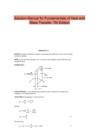 Textbook Guides
Solution Manual for Fundamentals of Heat and Mass Transfer, 7th Edition
Mechanical Engineering
2638 pagesMay 2025 Textbook Guides
Solution Manual for Engineering Mechanics Dynamics, 13th Edition
Mechanical Engineering
1360 pages123downloadsFeb 2025 Textbook Guides
Solution Manual For Introduction To Engineering Experimentation, 3rd Edition
Mechanical Engineering
298 pages99downloadsFeb 2025 Textbook Guides
Solution Manual for Mechanics of Materials SI, 9th Edition
Mechanical Engineering
1598 pages91downloadsFeb 2025 Textbook Guides
Solution Manual for Engineering Mechanics: Dynamics, 2nd Edition
Mechanical Engineering
41 pages82downloadsFeb 2025 Textbook Guides
Solution Manual for Finite Element Analysis: Theory and Application with ANSYS, 5th Edition
Mechanical Engineering
426 pages53downloadsFeb 2025 Textbook Guides
Solution Manual For Modern Compressible Flow: With Historical Perspective, 3rd Edition
Mechanical Engineering
362 pages52downloadsFeb 2025 Certification Guides
Biofluid Mechanics: An Introduction to Fluid Mechanics, Macrocirculation, and Microcirculation, 3rd Edition (2021)
Mechanical Engineering
172 pages48downloadsFeb 2025
Study this document with CramX
Once it is in your library, every tool can work from it.