

Solution Manual for Materials for Civil and Construction Engineers, 4th Edition
- Civil Engineering
- 136 pages
- Shared May 2025
Simplify your textbook learning with Solution Manual for Materials for Civil and Construction Engineers, 4th Edition, providing step-by-step solutions to every chapter.
Preview 16 of 136 pages
See the first 16 pages exactly as they appear in the document.
Page 1 Read page 1 as text
MATERIALS FOR CIVIL AND CONSTRUCTION ENGINEERS 4 th Edition Michael S. Mamlouk Arizona State University John P. Zaniewski West Virginia University Solution s Manual
Page 2 Page 3 Read page 3 as text
1 CHAPTER 1. MATERIALS ENGINEERING CONCEPTS 1.2. Strength at rupture = 45 ksi Toughness = (45 x 0.003) / 2 = 0.0675 ksi 1.3. A = 0.6 x 0.6 = 0.36 in 2 = 50,000 / 0.36 = 138,888.9 psi a = 0.007 / 2 = 0.0035 in/in l = -0.001 / 0.6 = -0.0016667 in/in E = 138,888.9 / 0.0035 = 39,682,543 psi = 39,683 ksi = 0.00166667 / 0.0035 = 0.48 1.4. A = 201.06 mm 2 = 0.945 GPa A = 0.002698 m/m L = 0.000625 m/m - E = 350.3 GPa = 0.23 1.5. A = d 2 /4 = 28.27 in 2 P / A = -150,000 / 28.27 in 2 = -5.31 ksi E = = 8000 ksi A E = -5.31 ksi / 8000 ksi = -0.0006631 in/in L A L o = -0006631 in/in (12 in) = -0.00796 in L f = L + L o = 12 in – 0.00796 in = 11.992 in L / A = 0.35 L d / d o = A = -0.35 (-0.0006631 in/in) = 0.000232 in/in d L d o = 0.000232 (6 in) = 0.00139 in d f = d + d o = 6 in + 0.00139 in = 6.00139 in 1.6. A = d 2 /4 = 0.196 in 2 P / A = 2,000 / 0.196 in = 10.18 ksi 2 (Less than the yield strength. Within the elastic region) E = = 10,000 ksi A E = 10.18 ksi / 10,000 ksi = 0.0010186 in/in L A L o = 0.0010186 in/in (12 in) = 0.0122 in L f = L + L o = 12 in + 0.0122 in = 12.0122 in L / A = 0.33 L d / d o = A = -0.33 (0.0010186 in/in) = -0.000336 in/in d L d o = -0.000336 (0.5 in) = -0.000168 in d f = d+ d o = 0.5 in - 0.000168 in = 0. 49998 in
Page 4 Read page 4 as text
2 1.7. L x =30 mm, L y = 60 mm, L z = 90 mm x = y = z = = 100 MPa E = 70 GPa = 0.333 x = [ x - ( y + z ) ] /E x = [100 x 10 6 - 0.333 (100 x 10 6 + 100 x 10 6 )] / 70 x 10 9 = 4.77 x 10 -4 = y = z = L x = x L x = 4.77 x 10 -4 x 30 = 0.01431 mm L y = x L y = 4.77 x 10 -4 x 60 = 0.02862 mm L z = x L z = 4.77 x 10 -4 x 90 = 0.04293 mm V = New volume - Original volume = [(L x - L x ) (L y - L y ) (L z - L z )] - L x L y L z = (30 - 0.01431) (60 - 0.02862) (90 - 0.04293)] - (30 x 60 x 90) = 161768 - 162000 = -232 mm 3 1.8. L x =4 in, L y = 4 in, L z = 4 in x = y = z = = 15,000 psi E = 1000 ksi = 0.49 x = [ x - ( y + z ) ] /E x = [15 - 0.49 (15 + 15)] / 1000 = 0.0003 = y = z = L x = x L x = 0.0003 x 15 = 0.0045 in L y = x L y = 0.0003 x 15 = 0.0045 in L z = x L z = 0.0003 x 15 = 0.0045 in V = New volume - Original volume = [(L x - L x ) (L y - L y ) (L z - L z )] - L x L y L z = (15 - 0.0045) (15 - 0.0045) (15 - 0.0045)] - (15 x 15 x 15) = 3371.963 - 3375 = -3.037 in 3 1.9. = 0.3 x 10 -16 3 At = 50,000 psi, = 0.3 x 10 -16 (50,000) 3 = 3.75 x 10 -3 in./in. Secant modulus = 50,000 3.75 x 10 3 = 1.33 x 10 7 psi 2 d 0.9 x 10 -16 d At = 50,000 psi, d d 0.9 x 10 -16 (50,000) 2 = 2.25 x 10 -7 in. 2 /lb Tangent modulus = d d 1 2.25 x 10 7 = 4.44x10 6 psi
Page 5 Read page 5 as text
3 1.11. lateral = 1 3.25 x 10 4 = -3.25 x 10 -4 in./in. axial = 2 10 2 3 x = 1 x 10 -3 in./in. = lateral axial 3.25 x 10 1 x 10 4 3 = 0.325 1.12. axial = 0.05 / 50 = 0.001 in./in. lateral = - x axial = -0.33 x 0.001 = -0.00303 in./in. d = lateral x d 0 = - 0.00825 in. (Contraction) 1.13. L = 380 mm D = 10 mm P = 24.5 kN = P/A = P/ r 2 = 24,500 N/ (5 mm) 2 = 312,000 N/mm 2 = 312 Mpa The copper and aluminum can be eliminated because they have stresses larger than their yield strengths as shown in the table below. For steel and brass, = AE PL 24,500 lbx 380 mm mm ) E ( kPa E ( MPa 118,539 2 (5 ) ) mm Material Elastic Modulus (MPa) Yield Strength (MPa) Tensile Strength (MPa) Stress (MPa) (mm) Copper 110,000 248 289 312 Al. alloy 70,000 255 420 312 Steel 207,000 448 551 312 0.573 Brass alloy 101,000 345 420 312 1.174 The problem requires the following two conditions: a . No plastic deformation Stress < Yield Strength b . Increase in length, < 0.9 mm The only material that satisfies both conditions is steel . 1.14. This stress is less than the yield strengths of all metals listed.
Page 6 Read page 6 as text
4 Material E (ksi) Yield Strength (ksi) Tensile Strength (ksi) L (in.) Steel alloy 1 26,000 125 73 0.014 Steel alloy 2 29,000 58 36 0.013 Titanium alloy 16,000 131 106 0.023 Copper 17,000 32 10 0.022 Only the steel alloy 1 and steel alloy 2 have elongation less than 0.018 in. 1.15 . This stress is less than the yield strengths of all metals listed. Material E (GPa) Yield Strength (MPa) Tensile Strength (MPa) L (mm) Steel alloy 1 180 860 502 0.378 Steel alloy 2 200 400 250 0.340 Titanium alloy 110 900 730 0.618 Copper 117 220 70 0.581 Only the steel alloy 1 and steel alloy 2 have elongation less than 0.45 mm. 1.16. a. E = / = 40,000 / 0.004 = 10 x 10 6 psi b. Tangent modulus at a stress of 45,000 psi is the slope of the tangent at that stress = 4.7 x 10 6 psi c. Yield stress using an offset of 0.002 strain = 49,000 psi d. Maximum working stress = Failure stress / Factor of safety = 49,000 / 1.5 = 32,670 psi 1.17. a. Modulus of elasticity within the linear portion = 20,000 ksi. b. Yield stress at an offset strain of 0.002 in./in. 70.0 ksi c. Yield stress at an extension strain of 0.005 in/in. 69.5 ksi d. Secant modulus at a stress of 62 ksi. 18,000 ksi e. Tangent modulus at a stress of 65 ksi. 6,000 ksi
Page 7 Read page 7 as text
5 1.18. a. Modulus of resilience = the area under the elastic portion of the stress strain curve = ½(50 x 0.0025) 0.0625 ksi b. Toughness = the area under the stress strain curve (using the trapezoidal integration technique) 0.69 ksi c = 40 ksi , this stress is within the elastic range, therefore, E = 20,000 ksi axial = 40/20,000 = 0.002 in./in. = 0.002 0.00057 axial lateral = 0.285 d. The permanent strain at 70 ksi = 0.0018 in./in. 1.19. Material A Material B a. Proportional limit 51 ksi 40 ksi b. Yield stress at an offset strain of 0.002 in./in. 63 ksi 52 ksi c. Ultimate strength 132 ksi 73 ksi d. Modulus of resilience 0.065 ksi 0.07 ksi e. Toughness 8.2 ksi 7.5 ksi f. Material B is more ductile as it undergoes more deformation before failure 1.20. Assume that the stress is within the linear elastic range. 10 . E 0.3 x 16,000 . l E 480 ksi Thus > yield Therefore, the applied stress is not within the linear elastic region and it is not possible to compute the magnitude of the load that is necessary to produce the change in length based on the given information. ,
Page 8 Read page 8 as text
6 1.21. Assume that the stress is within the linear elastic range. 250 . E 7.6 x 105,000 . l E 3,192 MPa Thus > yield Therefore, the applied stress is not within the linear elastic region and it is not possible to compute the magnitude of the load that is necessary to produce the change in length based on the given information. 1.22. At = 60,000 psi, = / E = 60,000 / (30 x 10 6 ) = 0.002 in./in. a. For a strain of 0.001 in./in.: = E = 0.001 x 30 x 10 6 = 30,000 psi ( for both i and ii) b. For a strain of 0.004 in./in.: = 60,000 psi (for i) = 60,000 + 2 x 10 6 (0.004 - 0.002) = 64,000 psi ( for ii) 1.23. a. Slope of the elastic portion = 600/0.003 = 2x10 5 MPa Slope of the plastic portion = (800-600)/(0.07-0.003) = 2,985 MPa Strain at 650 MPa = 0.003 + (650-600)/2,985 = 0.0198 m/m Permanent strain at 650 MPa = 0.0198 – 650/(2x10 5 ) = 0.0165 m/m b. Percent increase in yield strength = 100(650-600)/600 = 8.3% c. The strain at 625 MPa = This strain is elastic. 625/(2x10 5 ) = 0.003125 m/m 1.24 . a. 0.000399 Pa = 398 MPa b.
Page 9 Read page 9 as text
7 1.25 . a. 37,266.667 psi b. 1.26 . 4 = F - d d E 1.27 . 4 = F - d d E 1.28. See Sections 1.2.3, 1.2.4 and 1.2.5.
Page 10 Read page 10 as text
8 1.29. The stresses and strains can be calculated as follows: = P/A o = 150 / ( x 2 2 ) = 11.94 psi = (H o -H)/H o = (6-H)/6 The stresses and strains are shown in the following table: Time (min.) H (in.) Strain Stress (psi) (in./in.) 0 6 0.00000 11.9366 0.01 5.9916 0.00140 11.9366 2 5.987 0.00217 11.9366 5 5.9833 0.00278 11.9366 10 5.9796 0.00340 11.9366 20 5.9753 0.00412 11.9366 30 5.9725 0.00458 11.9366 40 5.9708 0.00487 11.9366 50 5.9696 0.00507 11.9366 60 5.9688 0.00520 11.9366 60.01 5.9772 0.00380 0.0000 62 5.9807 0.00322 0.0000 65 5.9841 0.00265 0.0000 70 5.9879 0.00202 0.0000 80 5.9926 0.00123 0.0000 90 5.9942 0.00097 0.0000 100 5.9954 0.00077 0.0000 110 5.9959 0.00068 0.0000 120 5.9964 0.00060 0.0000
Page 11 Read page 11 as text
9 a. Stress versus time plot for the asphalt concrete sample 0 2 4 6 8 10 12 14 0 50 100 150 Stress, psi Time, minutes Strain versus time plot for the asphalt concrete sample b. Elastic strain = 0.0014 in./in. c. The permanent strain at the end of the experiment = 0.0006 in./in. d. The phenomenon of the change of specimen height during static loading is called creep while the phenomenon of the change of specimen height during unloading called is called recovery.
Page 12 Read page 12 as text
10 1.30. See Figure 1.12(a). 1.31 . a. For F F o : = F.t / For F > F o , movement b. For F F o : = F / M For F > F o : = F / M + (F - F o ) t / 1.32 . See Section 1.2.7. 1.34. a. For P = 5 kN Stress = P / A = 5000 / ( x 5 2 ) = 63.7 N/mm 2 = 63.7 MPa Stress / Strength = 63.7 / 290 = 0.22 From Figure 1.16, an unlimited number of repetitions can be applied without fatigue failure. b. For P = 11 kN Stress = P / A = 11000 / ( x 5 2 ) = 140.1 N/mm 2 = 140.1 MPa Stress / Strength = 140.1 / 290 = 0.48 From Figure 1.16, N 700 1.35 . See Section 1.2.8. 1.36. Material Specific Gravity Steel 7.9 Aluminum 2.7 Aggregates 2.6 - 2.7 Concrete 2.4 Asphalt cement 1 - 1.1 1.37 . See Section 1.3.2. 1.38. L = L x T x L = 12.5E-06 x (115-15) x 200/1000 = 0.00025 m = 250 microns Rod length = L + L = 200,000+ 250 = 200,250 microns Compute change in diameter linear method d = d x T x d = 12.5E-06 x (115-15) x 20 = 0.025 mm Final d = 20.025 mm
Page 13 Read page 13 as text
11 Compute change in diameter volume method V = V x T x V = (3 x 12.5E-06) x (115-15) x (10/1000) 2 x 200/1000 = 2.3562 x 10 11 m 3 Rod final volume = V + V = r 2 L + V x + 2.3562 x 10 11 = 6.31 x 10 13 m 3 Final d = 20.025 mm There is no stress acting on the rod because the rod is free to move. 1.39. Since the rod is snugly fitted against two immovable nonconducting walls, the length of the rod will not change, L = 200 mm From problem 1.25, L = 0.00025 m = L / L = 0.00025 / 0.2 = 0.00125 m/m = E = 0.00125 x 207,000 = 258.75 MPa The stress induced in the bar will be compression. 1.40. a. The change in length can be calculated using Equation 1.9 as follows: L = L x T x L = 1.1E-5 x (5 - 40) x 4 = -0.00154 m b. The tension load needed to return the length to the original value of 4 meters can be calculated as follows: = L / L = -0.00154/ 4 = -0.000358 m/m = E = -0.000358 x 200,000 = -77 MPa P = x A = -77 x (100 x 50) = -385,000 N = -385 kN (tension) c. Longitudinal strain under this load = 0.000358 m/m 1.41. If the bar was fixed at one end and free at the other end, the bar would have contracted and no stresses would have developed. In that case, the change in length can be calculated using Equation 1.9 as follows. L = L x T x L = 0.000005 x (0 - 100) x 50 = -0.025 in. = L / L = 0.025 / 50 = 0.0005 in./in. Since the bar is fixed at both ends, the length of the bar will not change. Therefore, a tensile stress will develop in the bar as follows. = E = -0.0005 x 5,000,000 = -2,500 psi Thus, the tensile strength should be larger than 2,500 psi in order to prevent cracking. 1.43. See Section 1.7.
Page 14 Read page 14 as text
12 1.44. See Section 1.7.1 1.45. H o : 32.4 MPa H 1 : 32.4 MPa = 0.05 T o = x = -3 ( / n ) Degree of freedom = = n - 1 = 15 From the statistical t-distribution table, T , = T 0.05, 15 = -1.753 T o < T , Therefore, reject the hypothesis. The contractor’s claim is not valid. 1.46. H o : 5,000 psi H 1 : 5,000 psi = 0.05 T o = x = -2.236 ( / n ) Degree of freedom = = n - 1 = 19 From the statistical t-distribution table, T , = T 0.05, 19 = -1.729 T o < T , Therefore, reject the hypothesis. The contractor’s claim is not valid. 1.47. psi x n x x i i n i 5,698.25 20 113,965 20 20 1 1 i x n x x s i i n i i 571.35 1 20 5698.25) ( 1 ) ( 1/ 2 20 1 2 1/ 2 1 2 psi Coefficient of Variation = 10.03% 5698.25 571.35 100 100 s x b. The control chart is shown below.
Page 15 Read page 15 as text
13 The target value is any value above the specification limit of 5,000 psi. The plant production is meeting the specification requirement.
Page 16 Read page 16 as text
14 1.48. a. i 20 110.7 20 20 i 1 1 i n i x n x x 5.5 % 1/ 2 20 1 2 1/ 2 1 2 1 20 5.5) ( 1 ) ( i i n i i x n x x s 0.33 % s 5.5 0.33 100 100 x C 6 % b. The control chart is shown below. The control chart shows that most of the samples have asphalt content within the specification limits. Only few samples are outside the limits. The plot shows no specific trend, but large variability especially in the last several samples. 1.49 . See Section 1.8.2. 1.50 . See Section 1.8.
120 more pages in the full document
Unlock it once and it stays in your library, ready to chat with or turn into flashcards.
Unlock the full documentMore Civil Engineering study materials
See all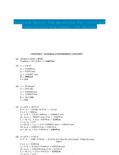 Textbook Guides
Solution Manual For Materials For Civil And Construction Engineers, 3rd Edition
Civil Engineering
105 pagesMay 2025 Textbook Guides
Solution Manual for Transportation Engineering and Planning, 3rd Edition
Civil Engineering
78 pages92downloadsFeb 2025 Textbook Guides
Reinforced Concrete Design, 9th Edition Solution Manual
Civil Engineering
198 pages65downloadsFeb 2025 Exam Guides
Principles Of Foundation Engineering, 8th Edition Test Bank
Civil Engineering
166 pages49downloadsFeb 2025 Textbook Guides
Solution Manual for A First Course in the Finite Element Method, 6th Edition
Civil Engineering
644 pagesMay 2025 Past Exams
The CE Shop Construction Final Exam With Answers (100 Solved Questions)
Civil Engineering
55 pagesMay 2025 Textbook Guides
Solution Manual for Structural Steel Design, 6th Edition
Civil Engineering
511 pagesMay 2025 Textbook Guides
Solution Manual For Structural Wood Design: ASD/LRFD, 2nd Edition
Civil Engineering
268 pagesMay 2025
Study this document with CramX
Once it is in your library, every tool can work from it.