Solution Manual for The Finite Element Method: Basic Concepts and Applications with MATLAB, MAPLE, and COMSOL,, 3rd Edition

Preview (16 of 402 Pages)

100%

Solution Manual for The Finite Element Method: Basic Concepts and Applications with MATLAB, MAPLE, and COMSOL,, 3rd Edition - Page 1 preview image

Loading page ...

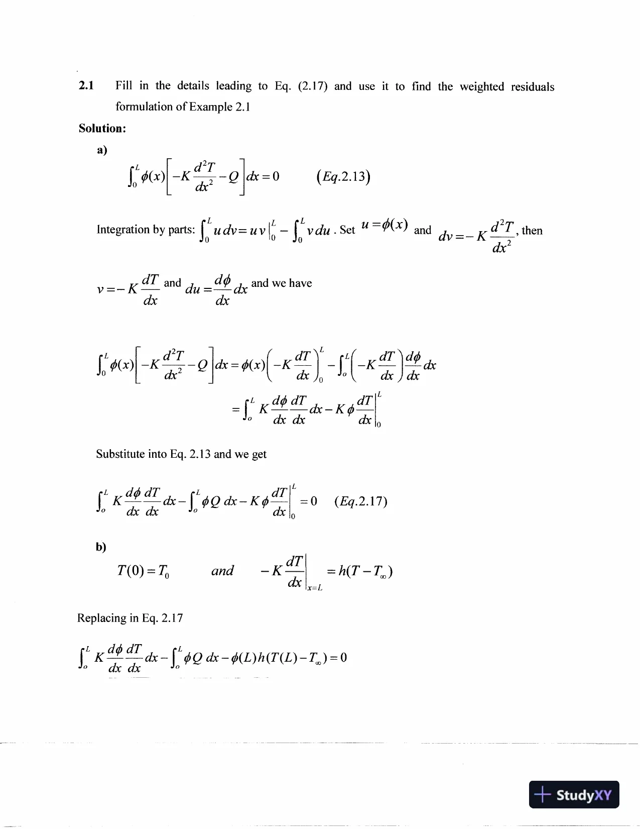
2.1Fillin thedetailsleading toEq. (2.17)anduseit tofindtheweighted residualsformulation of Example 2.1Solution:a)dxck = 0(Eq.l.U)Integration by parts:udv=uv'%Jw.Set" - ^ Wand^ ^ ^ _ ^ ^ , t h e nv=-K^^"'^ du=^dxdxdxd^Tdx^dx - (j>{x) -KVdJ^dxdx dx-KdTLd^dx dxdxSubstitute into Eq. 2.13 and we get°dx dxdx= 0{Eq.lAl)b)7(0) =and-K dTdxx=LKT-TJReplacing in Eq. 2.17K dx dx dx-^Qdx-^(L)h(T(L)-TJ= 0

Solution Manual for The Finite Element Method: Basic Concepts and Applications with MATLAB, MAPLE, and COMSOL,, 3rd Edition - Page 2 preview image

Loading page ...

Solution Manual for The Finite Element Method: Basic Concepts and Applications with MATLAB, MAPLE, and COMSOL,, 3rd Edition - Page 3 preview image

Loading page ...

2.2Use Eq. (2.17) to find the weighted residuals formulation of Eqs. (2.1)the heat flux q.Solution:- (2.3) in terms ofcL^d(l>dTK•''^dxdxrLdx-^Qdx+ ^-KdT_dx=0The heat flux term at x = L must be zero, anddT-KdxHencex=QL^dldT^^^^f i ^ ^dx + ^(0)q^dxdx•'^

Solution Manual for The Finite Element Method: Basic Concepts and Applications with MATLAB, MAPLE, and COMSOL,, 3rd Edition - Page 4 preview image

Loading page ...

2.3Obtain expression (2.30).Solution:The weighted residuals form for the second term is>(X)dx = 0After integration by parts on the first termKdx dxdx-ipQ dx + ^ •K dT_dx= 0L/2Note: The boundary terms are set to zero i f no fluxes are prescribed.The functionsfor element 2 areJ-/LetT{x) = -{L-x)a,+j(x-LI2)a,{Eq.2.\9)Using E q . 2.281L22 "dx<.L/22_ L _LL_a.L/2-(x-L/2)^ Ldx-Or4KrL" 1- Idx-'^212QrL<L/2- 11a.L 'L/2(x-L/2)<>—<0y0VJ0Integrating we have2K'1-f<« 21> dx-< 00L- 111^3,4h/21

Solution Manual for The Finite Element Method: Basic Concepts and Applications with MATLAB, MAPLE, and COMSOL,, 3rd Edition - Page 5 preview image

Loading page ...

Consider the equation+ w + x = 0,0 < j c < lwith w(0) = u ( l ) = 0.Assume an approximation foru{x)=i(x) with ^ ( x ) = x ( l -The residual isR{u, x) - -2a^+a ,- x ) ] +Xand the weightWi{x)=(j) \{x)= JC(1 -x).Find the solution from the following integral.Solution:rlrlW{x) R(u, x)dx=x(l - x)(-2a^+ a^x(l -x)+ x)dx = 0Orrl0W(x) R(u, x)ck=^ (-2a^x+ (3a, + l)x^ -2a^+ l)x^ +a^x"^)ck = 0-a,4 - - ( 3 a + l ) - - ( 2 a , + l ) + - a=—+— = 013V1^4 V1;^110'125therefore5' 1 818Compare with the exact solution given byu (x)XsinlEvaluating atx=l/2u{VI7)—0.069444^^^^"^^^^error.w * ( l / 2 ) = 0.069747

Solution Manual for The Finite Element Method: Basic Concepts and Applications with MATLAB, MAPLE, and COMSOL,, 3rd Edition - Page 6 preview image

Loading page ...

2.5Use the weak statement formulation to find solutions to theequationdx"w(0) = 0,= 1,0 < j c < ldudx(a)Usinglinearinterpolationfunctions,asexplainedinSection2.3,use(i) oneelement and (ii) twoelements.(b)Using simple polynomial functions that satisfy the boundary conditions at the left-hand side, i.e.,(i)u(x) = a\x,hence ^ i ( x ) =W\{x) = x(ii)u{x)= (afix+a2X^, hence(f>\{x) = Wx{x) = x,(l>2{x)=W2ix)-^x\(c)Using circular functions that satisfy the boundaryconditions at the left-handside,i.e.,(i)u{x)= a/ sin(n/2Lx)(ii)u{x)= «y sin(n/2Lx)+aa2sin(3n/2Lx)(d) Find the analytical solution and compare with results from (a), (b) and (c).Solutiona) The residual function is]^(u^x)=^ +1The weak form after integration by parts isdx^f dWdu^ dx-du+ Wdx- -W—Jo^ dxdxJdx=0i)One element solutionu{x)= ( l - x ) ^ ! +X<32j ;[ - 1\\dx<dx-'00[ - 1\\dx<dx-'.— <>1 _ [ - 1\\dx<J O10Integratingflf]-<22 =- 1 / 2—a^^+ ^2 = 1 / 2sincea | = 0thena 2 = l / 2oru(x)=x/2

Solution Manual for The Finite Element Method: Basic Concepts and Applications with MATLAB, MAPLE, and COMSOL,, 3rd Edition - Page 7 preview image

Loading page ...

Two element solution. Element 1:H/ 2~-2~[ - 22]dx\rl/2~l-2x~0]ol" 2- 2 "- 1 / 4[ - 22]dx\> +dx-<>— <>or<>.0_ 2 _[^2J0_2 x_ojOJ_ - 22 _- 1 / 4Element 2^ 2 = 2 ( l - x )^ 3 - 2 ( x - l / 2 )r - 9 i- 22]dx1/2- 22a-,1/22 ( 1 - x )2 ( x - l / 2 ) JAssembledx-the>or2- 2- 22^2«3- 1 / 43 / 4elements" 2- 20 "- 1 / 4 ^- 24- 2<«2- 1 / 2 >0- 22 _3 / 4>sincea^^Qwegeta2=ll^anda^=lf2u(x)=3 x - lx / 40 < x < l / 2l / 2 < x < lb)Using polynomialsi)^ j = xu[x)= a^x(la^+ x)dx-l= 0,a^=\l2,i / ( x ) = x / 2 , same as using one element.ii)^ i - x,(l>2=x^'u{x)= a^x + a2X^F o r W = ^ |r[1 • (<3i + 2 « 2 ^ ) +- 1 = 0r i rF o r W = ^ 2Jo• ( a , + 2 a 2 x ) + x ^ k/x - 1 = 0T h e system becomes^1+^2= 1 / 24a i+—^9= 2 / 3orc)a= 0,^2 = 1 / 2<3«(iw ( x ) = X ^ / 2

Solution Manual for The Finite Element Method: Basic Concepts and Applications with MATLAB, MAPLE, and COMSOL,, 3rd Edition - Page 8 preview image

Loading page ...

Using circular functionsi)^ } = sin— Xv2J,u {x)= aisin— Xv2y,d>\ — cos^2— XV 2y^2— f l jcos;7r— X2+ sm— Xv2yti6c-sin— Xv 2/- 00Use the identities21cosaxdx=—(si naxcosax- ax)and2a• • sinVn— X2cos8; T—Xv 2,1/+0^2cosn— XV2))- s m— Xv 2ydudx27tsin— Xcos— XUJ;rl 2j.Thei= 0orhencea, » 0.295andM ( X) = 0.295 s i n— XV 2Jii)^ 2= s mF o rr = ^ :Forr =^2 :Xd)^ 2f3^sin—X+A TsinXsinl 2yI2jcos3 — c o s— XV 2yflj cosV— Xv2y+ <3r2 cosX+ sin3 — X2^1cosV+ ^2cos3;r— Xv 2y( i r - s i n•XJ J+ sin3;7-•X2(ir-sin/Vdx- 003;r\du—X1Jdx2— flfj+ 0 •(32 H1 = 0(ajisunchanged)8n97r^20 - a ,+—+ 1 = 0.fl2~-0-109and^8^3;r^w ( x ) « 0.295 s i n- 0 . 1 0 9 s i n— Xv2yAnalytical3;rXsolution-.2= 1, integratingw ( x ) =—+ CjX +C2and applying boundary conditionsu( x ) =

Solution Manual for The Finite Element Method: Basic Concepts and Applications with MATLAB, MAPLE, and COMSOL,, 3rd Edition - Page 9 preview image

Loading page ...

Notice that all the approximations are exact at x = 1/2, and the Galerkin approximations using x2andXboth yield the exact solution. Also notice that the boundary condition at x = 1 is satisfiedonly approximately. I n case a), the first solution gives^dx_ i . and the second solution gives2dudxJC-l_ ^which is getting better.This point is discussed in more detail in problem 2.6.4

Solution Manual for The Finite Element Method: Basic Concepts and Applications with MATLAB, MAPLE, and COMSOL,, 3rd Edition - Page 10 preview image

Loading page ...

2.6Subdivide the interval 0 < x < Z into 10 linear elements, construct the element equationsfor four consecutive elements starting with element four, and show that none of theparameters aj is related to more than two additional parameters in the equations.Theonly ones involved being ai-i and a,+] (as a consequence of this, the final system of linearequations will involve a tri-diagonal matrix which is easy to solve).Solution:Foranelemente^^={x/Xj^<x<Xi^_^_^)theelementstiffnessmatrixisobtainedfromr^k+'i^.All the stiffness matrices must be equal, so let's calculate the firstdxdxone.A11^^ 1=1X^2=10Land after assembling1 0 ^thus1- 100r i / l OL- 12- 10K012- 110~ L10L00- 121010dx=- lOK0000000000- 10- 11a ,a-,a10a11• 1- 1- 11Note that each equation / involves only three unknownsand a^^^,so the stiffness matrixis tri-diagonal.

Solution Manual for The Finite Element Method: Basic Concepts and Applications with MATLAB, MAPLE, and COMSOL,, 3rd Edition - Page 11 preview image

Loading page ...

2.7The Rayleigh-Ritz formulationfor theproblemof solving Eq. (2.1) withboundaryconditions (2.2)and (2.3) can be stated as: Minimize the fiinctionalF{T)=£2dx-QT\dx-Tq.t=0over all functionsT{x)with square integrablefirst derivatives that satisfy Eq. (2.3) at x = Z.ApproximateT{x)using two linear elements as we did before and replace into Eq. (2.1)toobtainF{T) =F(«],ai, a^).Now minimizeF{a\, a^, ai)as a function of three variables.Show that the final system of equations is identical to Eq. (2.31), thus, in this case, theGalerkin method and the Rayleigh-Ritz method are equivalent.Solution:Element I :(b^=1X^L,2>2 = — XLrLIlKV— a, +—^2L^L^\-QJo2(1)Element2:22r2^1XVLJ2^K..2QL..a^+-xa2]fh-a^g= —(a2-ai)——(a^+a2)-a^qKL'LK_111222flnHQnL^L^\-Q2XL- x - 1La^\bc-a^q= —{a^-a2)— ; ^ ( « 2 + « 3 )(2)F(T)=(1)+ (2) = ^{a2-a,f+j{a^- «2 ) '( ^ i + 2^2+ «3 ) "^^/222 \F ( r )= F( a j , a 2 ,) =—(^fli-2(2,<32 +2^2-2fl2<^3 + ^3 jTheconditions for a minimum aredF_dF_dFda^5^2^^3_ Q thus{a,-a2)-^-q= 0LdF2Kda2LdFIKL(-flj+2^2"^^2)( a 3- a , ) - ^=0QLIn Matrix form2KL"1- 10""a2a- 12- 1<a22> + <0 >0- 1140- 1110which is identical to Eq. 2.31.

Solution Manual for The Finite Element Method: Basic Concepts and Applications with MATLAB, MAPLE, and COMSOL,, 3rd Edition - Page 12 preview image

Loading page ...

2.8Let us consider once more Problem 2.3 above.Assume that w(x) =aix^andWi(x) = x^,but this time use E q . (2.11) and proceed as in Problem 2.2 in order to obtain a solution.Show that this solution is identical to that obtained in Problem 2.3(b)(ii), and hence, theprocess of integration by parts does not introduce any changes.Solution:- 1dx =rlx\2a-\)dx= 0'23x'^— x a,21= 0,—a—= 0,a, = 1 / 2, w(;33'

Solution Manual for The Finite Element Method: Basic Concepts and Applications with MATLAB, MAPLE, and COMSOL,, 3rd Edition - Page 13 preview image

Loading page ...

2.9In example 2.2, first find the exact analytical solution, then calculate two more Galerkinapproximations usingSolution:Theanalyticalsolutionis^dWduii(^x) =—{^x-x^yTheGalerkinapproximationisdxdx-Wdx =0'u(x)=(3] sin;rx +sin27tx,= sinTTX,sinITTXa)rloL0 _cosTTxf^a^cosTTX+ lajcos 2;rx) - sinnx dx =0ITV^cosInxcosnx+ 2a2 cosInx)-sin 2-;rxtir = 0or—fli+0-a2= 0,a^=—u{x)- —sin ;rxn, <3«flf0 • ^1 + 2:7r ^2 +0 = 0,b)M(x) = aj sin:;rx + a2sin2;7rx+ a3sin3:7rx,f P j = s i n ; r x,W^^^VCLITIX,H^=sin3;TxWe only need to calculate,andremain the same due to the orthogonality of the sinefunctions.:3;r^ cos 3;rx(fl} cos;7rx+2^2 cos 2;rx4-3(33 cos 3 ; r x ) - s i n 3:^xr2'3;r'Tin",W3(x) =—3;r'*1.sin ;rx + —sin 3;rx27

Solution Manual for The Finite Element Method: Basic Concepts and Applications with MATLAB, MAPLE, and COMSOL,, 3rd Edition - Page 14 preview image

Loading page ...

3.1Repeat the development of expressions (3.7) to (3.12) using two linear elements to discretize the interval0<x<L.Then combinetheelement shape functionsto constructthe global shape functionsandcompare your result to that obtained using expressions (3.2) to (3.4) directly, withn = 2.Solution:LetT(x) = a + j3xwithTix^) = T-and7( ^ , ^ 1)=T-^^ •Hencea + fix^ = T-anda+ y^jc^^j = T^^j.Thereforea =andp—^+1andXRearrangingT{x) =x-x^^.Thisexpressionisvalidforanyelement, inr /N,(x)= \N2(X)={particular if we have two elementsN.(x)= \x-^-xyXj-x^J^X ^ X20otherwiseXX]^ X2 -XiyXo- XyX3 -X2yX |< X < X2X2 < X < X30otherwiseX-X2X2 <X < X30otherwiseN,{x)=IfXi =0,X2= 1 / 2andX3= L ThenN,(x)=- ^ ( Z - 2 x )0<x<L/20otherwise2— X0<x<L/2L-(L-x)L/2<x<LL0otherwise-{2x-L)L/2<x<LL0otherwiseThese expressions are exactly the same as those obtained from Eqs, 3.2 - 3.4.

Solution Manual for The Finite Element Method: Basic Concepts and Applications with MATLAB, MAPLE, and COMSOL,, 3rd Edition - Page 15 preview image

Loading page ...

3.2Show that if in Eq. (3.6) we replaceTn+i = T L,the boundary condition (2.3) is automatically satisfied.Solution:n+lnJFrom Eq. 3.6j ^ ^ ^ ) ^ ^(^)7^. ^ £j^j, ^^)T. + N^^^ (x)T^• Evaluate at X = X„^l = L . Then^ii^n+l)=^Mi = h2,...,nandiV„^.i(x„^i) =1• HenceT{x^^^)= Tj^.

Solution Manual for The Finite Element Method: Basic Concepts and Applications with MATLAB, MAPLE, and COMSOL,, 3rd Edition - Page 16 preview image

Loading page ...

3.3Derive expression (3.25) from (3.24) for cubic elements.Then find a relation between global and localreference systems such as the ones given in Figure 3.3 and 3.6 for linear and quadratic elements.Solution:Lethbe the size of the element. There are several ways to obtain the shape functions, the easiest is torecognize thatAT.(jc^.) = ^-y,N-^ (x^) = 1andN- (xj) =0if / ^ J .Sofor /• = 1, i\^i(0)= l ,N^(h/3)= N^(2h/3)= N^(h) =0and thereforeN^ix)must have the formTVj(x) = a(x-h/3Xx-2hl3)(x-h)and imposing(0) = 1we get ^ ^11?AT, (x) = —^ (x -/2/ 3)(x -Ih 13)(x - /z) = (1 - 3x /- 3x / 2/z)(l-xlh)2hahSimilarly we getN2(x) =-ax{x-2h/ 3)(x -/z),/3) = 1= y(-/? /3)(-2h13)so^ ^ ^ 7and iV2(x) = ^ x ( x - 2 / z / 3 ) ( x - ; 7 ) = — ( l - 3 x / 2 / z ) ( l - x / i ? 7 ) -^^2(^)^ 3 ( ^ )2h^2h^hare similarly obtained and given byM^i^x) = -—{\-3xlh){\-xlh)and N^{x) =--{\-Zxlh){\-3xl2h)2hhThe relation between the local and global system in elementis given byLocalGlobalNodeNodenumbersnumbers13i+l23i+233i+343i+4

Preview Mode

This document has 402 pages. Sign in to access the full document!

Report

Study Now!

Document Details

Related Documents

Precalculus - Polynomial and Rational Functions

Precalculus - Functions

Precalculus - Exponential and Logarithmic Functions

Math Word Problems - Translating Expressions

Math Word Problems - Equations

Algebra II – Word Problems

Algebra II – Sequences and Series

Algebra II - Segments Lines and Inequalities

Algebra II - Relations and Functions

Algebra II - Rational Expressions

Company

Explore

Study Tools