

Solution Manual for Manufacturing Processes for Engineering Materials, 6th Edition
- Mechanical Engineering
- 297 pages
- Shared May 2025
Master your textbook problems with Solution Manual for Manufacturing Processes for Engineering Materials, 6th Edition, providing comprehensive solutions and explanations.
Preview 16 of 297 pages
See the first 16 pages exactly as they appear in the document.
Page 1 Read page 1 as text
Manufacturing Processes for Engineering Materials, 6th ed. Serope Kalpakjian Steven R. Schmid
Page 2 Page 3 Read page 3 as text
Chapter 2 Fundamentals of the Mechanical Behavior of Materials QUESTIONS 2.1 Can you calculate the percent elongation of materials based only on the information given in Fig. 2.6? Ex plain. Recall that the percent elongation is defined by Eq. (2.6) on p. 35 and depends on the original gage length ( l o ) of the specimen. From Fig. 2.6 on p. 39, only the necking strain (true and engineering) and true fracture strain can be determined. Thus, we cannot calculate the per cent elongation of the specimen; also, note that the elongation is a function of gage length and increases with gage length. 2.2 Explain if it is possible for stress-strain curves in ten sion tests to reach 0% elongation as the gage length is increased further. The percent elongation of the specimen is a function of the initial and final gage lengths. When the specimen is being pulled, regardless of the original gage length, it will elongate uniformly (and permanently) until neck ing begins. Therefore, the specimen will always have a certain finite elongation. However, note that as the specimen’s gage length is increased, the contribution of localized elongation (that is, necking) will decrease, but the total elongation will not approach zero. 2.3 Explain why the difference between engineering strain and true strain becomes larger as strain increases. Is this phenomenon true for both tensile and compressive strains? Explain. The difference between the engineering and true strains becomes larger because of the way the strains are defined, respectively, as can be seen by inspecting Eqs. (2.1) and (2.9). This is true for both tensile and compressive strains. 2.4 Using the same scale for stress, the tensile true-stress true-strain curve is higher than the engineering stress- strain curve. Explain whether this condition also holds for a compression test. During a compression test, the cross-sectional area of the specimen increases as the specimen height de creases (because of volume constancy) as the load is in creased. Since true stress is defined as ratio of the load to the instantaneous cross-sectional area of the speci men, the true stress in compression will be lower than the engineering stress for a given load, assuming that friction between the platens and the specimen is negli gible. 2.5 Which of the two tests, tension or compression, re quires a higher capacity testing machine than the other? Explain. The compression test requires a higher capacity ma chine because the cross-sectional area of the specimen increases during the test, which is the opposite of a ten sion test. The increase in area requires a load higher than that for the tension test to achieve the same stress level. Furthermore, note that compression-test spec imens generally have a larger original cross-sectional area than those for tension tests, thus requiring higher forces. 2.6 Explain how the modulus of resilience of a material changes, if at all, as it is strained: (a) for an elastic, per fectly plastic material, and (b) for an elastic, linearly strain-hardening material. Recall that the modulus of resilience is given by Eq. (2.5) on p. 34 as S 2 y / (2 E ) . (a) If the material is perfectly plastic, then the yield strength does not in crease with strain - see Fig. 2.7c on p. 42. Therefore, the modulus of resilience is unchanged as the material is strained. (b) For a linear strain hardening material, the yield strength increases with plastic strain. Therefore the modulus of resilience will increase with strain. 1
Page 4 Read page 4 as text
2.7 If you pull and break a tensile-test specimen rapidly, where would the temperature be the highest? Explain why. Since temperature rise is due to the work input, the temperature will be highest in the necked region be cause that is where the strain, hence the energy dissi pated per unit volume in plastic deformation, is high est. 2.8 Comment on the temperature distribution if the speci men in Question 2.7 is pulled very slowly. If the specimen is pulled very slowly, the temperature generated will be dissipated throughout the specimen and to the environment. Thus, there will be no ap preciable temperature rise anywhere, particularly with materials with high thermal conductivity. 2.9 In a tension test, the area under the true-stress-true strain curve is the work done per unit volume (the spe cific work). Also, the area under the load-elongation curve represents the work done on the specimen. If you divide this latter work by the volume of the spec imen between the gage marks, you will determine the work done per unit volume (assuming that all defor mation is confined between the gage marks). Will this specific work be the same as the area under the true- stress-true-strain curve? Explain. Will your answer be the same for any value of strain? Explain. If we divide the work done by the total volume of the specimen between the gage lengths, we obtain the av erage specific work throughout the specimen. How ever, the area under the true stress-true strain curve represents the specific work done at the necked (and fractured) region in the specimen where the strain is a maximum. Thus, the answers will be different. How ever, up to the onset of necking (instability), the specific work calculated will be the same. This is because the strain is uniform throughout the specimen until neck ing begins. 2.10 The note at the bottom of Table 2.4 states that as tem perature increases, C decreases and m increases. Ex plain why. The value of C in Table 2.4 on p. 46 decreases with tem perature because it is a measure of the strength of the material. The value of m increases with temperature because the material becomes more strain-rate sensi tive, due to the fact that the higher the strain rate, the less time the material has to recover and recrystallize, hence its strength increases. 2.11 You are given the K and n values of two different mate rials. Is this information sufficient to determine which material is tougher? If not, what additional informa tion do you need, and why? Although the K and n values may give a good esti mate of toughness, the true fracture stress and the true strain at fracture are required for accurate calculation of toughness. The modulus of elasticity and yield stress would provide information about the area under the elastic region; however, this region is very small and is thus usually negligible with respect to the rest of the stress-strain curve. 2.12 Modify the curves in Fig. 2.7 to indicate the effects of temperature. Explain your changes. These modifications can be made by lowering the slope of the elastic region and lowering the general height of the curves. See, for example, Fig. 2.9 on p. 43. 2.13 Using a specific example, show why the deformation rate, say in m/s, and the true strain rate are not the same. The deformation rate is the quantity v in Eqs. (2.16) and (2.17). Thus, when v is held constant during de formation (hence a constant deformation rate), the true strain rate will vary ( l increases), whereas the engineer ing strain rate will remain constant. Hence, the two quantities are not the same. 2.14 It has been stated that the higher the value of m , the more diffuse the neck is, and likewise, the lower the value of m , the more localized the neck is. Explain the reason for this behavior. As discussed in Section 2.2.7, with high m values, the material stretches to a greater length before it fails; this behavior is an indication that necking is delayed with increasing m . When necking is about to begin, the necking region’s strength with respect to the rest of the specimen increases, due to strain hardening. However, the strain rate in the necking region is also higher than in the rest of the specimen, because the material is elon gating faster there. Since the material in the necked re gion becomes stronger as it is strained at a higher rate, the region exhibits a greater resistance to necking. The increase in resistance to necking thus depends on the magnitude of m . As the tension test progresses, neck ing becomes more diffuse , and the specimen becomes longer before fracture; hence, total elongation increases with increasing values of m . As expected, the elonga tion after necking ( postuniform elongation ) also increases with increasing m . It has been observed that the value of m decreases with metals of increasing strength. 2.15 Explain why materials with high m values, such as hot glass and silly putty, when stretched slowly, undergo large elongations before failure. Consider events tak ing place in the necked region of the specimen. The answer is similar to Answer 2.14 above. 2.16 Assume that you are running four-point bending tests on a number of identical specimens of the same length and cross-section, but with increasing distance be tween the upper points of loading (see Fig. 2.19b). What changes, if any, would you expect in the test re sults? Explain. 2
Page 5 Read page 5 as text
As the distance between the upper points of loading in Fig. 2.19b increases, the magnitude of the bending moment decreases. However, the volume of material subjected to the maximum bending moment (hence to maximum stress) increases. Thus, the probability of failure in the four-point test increases as this distance increases. 2.17 Would Eq. (2.10) hold true in the elastic range? Explain. Note that this equation is based on volume constancy, i.e., A o l o = Al . We know, however, that because the Poisson’s ratio ν is less than 0.5 in the elastic range, the volume is not constant in a tension test; see Eq. (2.47) on p. 71. Therefore, the expression is not valid in the elastic range. 2.18 Why have different types of hardness tests been devel oped? How would you measure the hardness of a very large object? There are several basic reasons: 1. The overall hardness range of the materials 2. The hardness of their constituents; see Chapter 3; 3. The thickness of the specimen, such as bulk ver sus foil 4. The size of the specimen with respect to that of the indenter 5. The surface finish of the part being tested. 2.19 Which hardness tests and scales would you use for very thin strips of material, such as aluminum foil? Why? Because aluminum foil is very thin, the indentations on the surface must be very small so as not to affect test results. Suitable tests would be a microhardness test such as Knoop or Vickers under very light loads (see Fig. 2.20 on p. 54). The accuracy of the test can be validated by observing any changes in the surface appearance opposite to the indented side. 2.20 List and explain the factors that you would consider in selecting an appropriate hardness test and scale for a particular application. Hardness tests mainly have three differences: 1. type of indenter, 2. applied load, and 3. method of indentation measurement (depth or surface area of indentation, or rebound of inden ter). 2.21 In a Brinell hardness test, the resulting impression is found to be an ellipse. Give possible explanations for this result. There are several possible reasons for this phe nomenon, but the two most likely are anisotropy in the material and the presence of surface residual stresses in the material. 2.22 Referring to Fig. 2.20, the material for testers are either steel, tungsten carbide, or diamond. Why isn’t dia mond used for all of the tests? While diamond is the hardest material known, it would not, for example, be practical to make and use a 10-mm diamond indenter because the costs would be prohibitive. Consequently, a hard material such as those listed are sufficient for most hardness tests. 2.23 What role does friction play in a hardness test? Can high friction between a material and indenter affect a hardness test? Explain. The effect of friction has been found to be minimal. In a hardness test, most of the indentation occurs through plastic deformation, and there is very little sliding at the indenter-workpiece interface; see Fig. 2.23 on p. 58. 2.24 Describe the difference between creep and stress relax ation, giving two examples for each as they relate to engineering applications. Creep is the permanent deformation of a part that is under a load over a period of time, usually occurring at elevated temperatures. Stress relaxation is the decrease in the stress level in a part under a constant strain. Ex amples of creep include: 1. turbine blades operating at high temperatures, and 2. high-temperature steam linesand furnace compo nents. Stress relaxation is observed when, for example, a rub ber band or a thermoplastic is pulled to a specific length and held at that length for a period of time. This phenomenon is commonly observed in rivets, bolts, and guy wires, as well as thermoplastic components. 2.25 Referring to the two impact tests shown in Fig. 2.26, explain how different the results would be if the speci mens were impacted from the opposite directions. Note that impacting the specimens shown in Fig. 2.26 on p. 61 from the opposite directions would subject the roots of the notches to compressive stresses, and thus they would not act as stress raisers. Thus, cracks would not propagate as they would when under ten sile stresses. Consequently, the specimens would basi cally behave as if they were not notched. 2.26 If you remove the layer ad from the part shown in Fig. 2.27d, such as by machining or grinding, which way will the specimen curve? ( Hint: Assume that the part in diagram (d) is composed of four horizontal springs held at the ends. Thus, from the top down, we have compression, tension, compression, and tension springs.) Since the internal forces will have to achieve a state of static equilibrium, the new part has to bow downward (i.e., it will hold water). Such residual-stress patterns 3
Page 6 Read page 6 as text
can be modeled with a set of horizontal tension and compression springs. Note that the top layer of the ma terial ad in Fig. 2.27d, which is under compression, has the tendency to bend the bar upward. When this stress is relieved (such as by removing a layer), the bar will compensate for it by bending downward. 2.27 Is it possible to completely remove residual stresses in a piece of material by the technique described in Fig. 2.29 if the material is elastic, linearly strain hardening? Ex plain. By following the sequence of events depicted in Fig. 2.29 on p. 64, it can be seen that it is not possi ble to completely remove the residual stresses. Note that for an elastic, linearly strain hardening material, σ c � will never catch up with σ t � . 2.28 Referring to Fig. 2.29, would it be possible to elimi nate residual stresses by compression? Assume that the piece of material will not buckle under the uniaxial compressive force. Yes, by the same mechanism described in Fig. 2.29 on p. 64. 2.29 List and explain the desirable mechanical properties for (a) an elevator cable; (b) a bandage; (c) a shoe sole; (d) a fish hook; (e) an automotive piston; (f) a boat pro peller; (g) a gas-turbine blade; and (h) a staple. The following are some basic considerations: (a) Elevator cable: The cable should not elongate elas tically to a large extent or undergo yielding as the load is increased. These requirements thus call for a material with a high elastic modulus and yield stress. (b) Bandage: The bandage material must be compli ant, that is, have a low stiffness, but have high strength in the membrane direction. Its inner sur face must be permeable and outer surface resis tant to environmental effects. (c) Shoe sole: The sole should be compliant for com fort, with a high resilience. It should be tough so that it absorbs shock and should have high fric tion and wear resistance. (d) Fish hook: A fish hook needs to have high strength so that it doesn’t deform permanently under load, and thus maintain its shape. It should be stiff (for better control during its use) and should be resistant the environment it is used in (such as salt water). (e) Automotive piston: This product must have high strength at elevated temperatures, high physical and thermal shock resistance, and low mass. (f) Boat propeller: The material must be stiff (to maintain its shape) and resistant to corrosion, and also have abrasion resistance because the pro peller encounters sand and other abrasive parti cles when operated close to shore. (g) Gas turbine blade: A gas turbine blade operates at high temperatures (depending on its location in the turbine); thus it should have high-temperature strength and resistance to creep, as well as to oxi dation and corrosion due to combustion products during its use. (h) Staple: The properties should be closely parallel to that of a paper clip. The staple should have high ductility to allow it to be deformed without fracture, and also have low yield stress so that it can be bent (as well as unbent when removing it) easily without requiring excessive force. 2.30 Make a sketch showing the nature and distribution of the residual stresses in Figs. 2.28a and b before the parts were cut. Assume that the split parts are free from any stresses. ( Hint: Force these parts back to the shape they were in before they were cut.) As the question states, when we force back the split portions in the specimen in Fig. 2.28a on p. 63, we in duce tensile stresses on the outer surfaces and com pressive on the inner. Thus the original part would, along its total cross section, have a residual stress dis tribution of tension-compression-tension. Using the same technique, we find that the specimen in Fig. 2.28b would have a similar residual stress distribution prior to cutting. 2.31 It is possible to calculate the work of plastic deforma tion by measuring the temperature rise in a workpiece, assuming that there is no heat loss and that the temper ature distribution is uniform throughout? If the spe cific heat of the material decreases with increasing tem perature, will the work of deformation calculated us ing the specific heat at room temperature be higher or lower than the actual work done? Explain. If we calculate the heat using a constant specific heat value in Eq. (2.62), the work will be higher than it ac tually is. This is because, by definition, as the specific heat decreases, less work is required to raise the work piece temperature by one degree. Consequently, the calculated work will be higher than the actual work done. 2.32 Explain whether or not the volume of a metal specimen changes when the specimen is subjected to a state of (a) uniaxial compressive stress and (b) uniaxial tensile stress, all in the elastic range. For case (a), the quantity in parentheses in Eq. (2.47) on p. 71 will be negative, because of the compressive stress. Since the rest of the terms are positive, the prod uct of these terms is negative and, hence, there will be a decrease in volume (This can also be deduced intu itively.) For case (b), it will be noted that the volume will increase. 2.33 It is relatively easy to subject a specimen to hydrostatic compression, such as by using a chamber filled with a liquid. Devise a means whereby the specimen (say, in 4
Page 7 Read page 7 as text
the shape of a cube or a round disk) can be subjected to hydrostatic tension, or one approaching this state of stress. (Note that a thin-walled, internally pressurized spherical shell is not a correct answer, because it is sub jected only to a state of plane stress.) Two possible answers are the following: 1. A solid cube made of a soft metal has all its six faces brazed to long square bars (of the same cross section as the specimen); the bars are made of a stronger metal. The six arms are then subjected to equal tension forces, thus subjecting the cube to equal tensile stresses. 2. A thin, solid round disk (such as a coin) and made of a soft material is brazed between the ends of two solid round bars of the same diameter as that of the disk. When subjected to longitudinal ten sion, the disk will tend to shrink radially. But be cause it is thin and its flat surfaces are restrained by the two rods from moving, the disk will be sub jected to tensile radial stresses. Thus, a state of tri axial (though not exactly hydrostatic) tension will exist within the thin disk. 2.34 Referring to Fig. 2.17, make sketches of the state of stress for an element in the reduced section of the tube when it is subjected to (a) torsion only; (b) torsion while the tube is internally pressurized; and (c) torsion while the tube is externally pressurized. Assume that the tube is a closed-end tube. These states of stress can be represented simply by re ferring to the contents of this chapter as well as the rel evant materials covered in texts on mechanics of solids. 2.35 A penny-shaped piece of soft metal is brazed to the ends of two flat, round steel rods of the same diameter as the piece. The assembly is then subjected to uniax ial tension. What is the state of stress to which the soft metal is subjected? Explain. The penny-shaped soft metal piece will tend to contract radially due to Poisson’s ratio; however, the solid rods to which it attached will prevent this from happening. Consequently, the state of stress will tend to approach that of hydrostatic tension. 2.36 A circular disk of soft metal is being compressed be tween two flat, hardened circular steel punches of hav ing the same diameter as the disk. Assume that the disk material is perfectly plastic and that there is no friction or any temperature effects. Explain the change, if any, in the magnitude of the punch force as the disk is being compressed plastically to, say, a fraction of its original thickness. Note that as it is compressed plastically, the disk will expand radially, because of volume constancy. An approximately donut-shaped material will then be pushed radially outward, which will then exert ra dial compressive stresses on the disk volume under the punches. The volume of material directly between the punches will now subjected to a triaxial compres sive state of stress. According to yield criteria (see Section 2.11), the compressive stress exerted by the punches will thus increase, even though the material is not strain hardening. Therefore, the punch force will increase as deformation increases. 2.37 A perfectly plastic metal is yielding under the stress state σ 1 , σ 2 , σ 3 , where σ 1 > σ 2 > σ 3 . Explain what happens if σ 1 is increased. Consider Fig. 2.32 on p. 70. Points in the interior of the yield locus are in an elastic state, whereas those on the yield locus are in a plastic state. Points outside the yield locus are not admissible. Therefore, an increase in σ 1 while the other stresses remain unchanged would require an increase in yield stress. This can also be de duced by inspecting either Eq. (2.38) or Eq. (2.39). 2.38 What is the dilatation of a material with a Poisson’s ra tio of 0.5? Is it possible for a material to have a Pois son’s ratio of 0.7? Give a rationale for your answer. It can be seen from Eq. (2.47) on p. 71 that the dilatation of a material with ν = 0 . 5 is always zero, regardless of the stress state. To examine the case of ν = 0 . 7 , consider the situation where the stress state is hydrostatic ten sion. Equation (2.47) would then predict contraction under a tensile stress, a situation that cannot occur. 2.39 Can a material have a negative Poisson’s ratio? Give a rationale for your answer. Solid material do not have a negative Poisson’s ratio, with the exception of some composite materials (see Chapter 10), where there can be a negative Poisson’s ratio in a given direction. 2.40 As clearly as possible, define plane stress and plane strain. Plane stress is the situation where the stresses in one of the direction on an element are zero; plane strain is the situation where the strains in one of the direction are zero. 2.41 What test would you use to evaluate the hardness of a coating on a metal surface? Would it matter if the coat ing was harder or softer than the substrate? Explain. The answer depends on whether the coating is rela tively thin or thick. For a relatively thick coating, con ventional hardness tests can be conducted, as long as the deformed region under the indenter is less than about one-tenth of the coating thickness. If the coat ing thickness is less than this threshold, then one must either rely on nontraditional hardness tests, or else use fairly complicated indentation models to extract the material behavior. As an example of the former, atomic force microscopes using diamond-tipped pyra mids have been used to measure the hardness of coat ings less than 100 nanometers thick. As an example of 5
Page 8 Read page 8 as text
the latter, finite-element models of a coated substrate being indented by an indenter of a known geometry can be developed and then correlated to experiments. 2.42 List the advantages and limitations of the stress-strain relationships given in Fig. 2.7. Several answers that are acceptable, and the student is encouraged to develop as many as possible. Two pos sible answers are: 1. There is a tradeoff between mathematical com plexity and accuracy in modeling material behav ior 2. Some materials may be better suited for certain constitutive laws than others 2.43 Plot the data in the inside front cover on a bar chart, showing the range of values, and comment on the re sults. By the student. An example of a bar chart for the elastic modulus is shown below. 0 100 200 300 400 500 Aluminum Copper Lead Magnesium Molybdenum Nickel Steels Stainless steels Titanium Tungsten Elastic modulus (GPa) Metallic materials 0 200 400 600 800 1000 1200 Ceramics Diamond Glass Rubbers Thermoplastics Thermosets Boron fibers Carbon fibers Glass fibers Kevlar fibers Spectra fibers Elastic modulus (GPa) Non-metallic materials Typical comments regarding such a chart are: 1. There is a smaller range for metals than for non metals; 2. Thermoplastics, thermosets and rubbers are or ders of magnitude lower than metals and other non-metals; 3. Diamond and ceramics can be superior to others, but ceramics have a large range of values. 2.44 A hardness test is conducted on as-received metal as a quality check. The results show indicate that the hard ness is too high, indicating that the material may not have sufficient ductility for the intended application. The supplier is reluctant to accept the return of the ma terial, instead claiming that the diamond cone used in the Rockwell testing was worn and blunt, and hence the test needed to be recalibrated. Is this explanation plausible? Explain. Refer to Fig. 2.20 on p. 54 and note that if an inden ter is blunt, then the penetration, t , under a given load will be smaller than that using a sharp indenter. This then translates into a higher hardness. The explanation is plausible, but in practice, hardness tests are fairly reliable and measurements are consistent if the test ing equipment is properly calibrated and routinely ser viced. 2.45 Explain why a 0.2% offset is used to obtain the yield strength in a tension test. The value of 0.2% is somewhat arbitrary and is used to set some standard. A yield stress, representing the transition point from elastic to plastic deformation, is difficult to measure. This is because the stress-strain curve is not linearly proportional after the propor tional limit, which can be as high as one-half the yield strength in some metals. Therefore, a transition from elastic to plastic behavior in a stress-strain curve is dif ficult to discern. The use of a 0.2% offset is a con venient way of consistently interpreting a yield point from stress-strain curves. 2.46 Referring to Question 2.45, would the offset method be necessary for a highly strained hardened material? Ex plain. The 0.2% offset is still advisable whenever it can be used, because it is a standardized approach for deter mining yield stress, and thus one should not arbitrarily abandon standards. However, if the material is highly cold worked, there will be a more noticeable ‘kink’ in the stress-strain curve, and thus the yield stress is far more easily discernable than for the same material in the annealed condition. 2.47 Explain why the hardness of a material is related to a multiple of the uniaxial compressive stress, since both involve compression of workpiece material. The hardness is related to a multiple of the uniaxial compressive stress, not just the uniaxial compressive stress, because: 6
Page 9 Read page 9 as text
1. The volume of material that is stressed is different - in a hardness test, the volume that is under stress is not just a cylinder beneath the inventor. 2. The stressed volume is constrained by the elas tic material outside of the indentation area. This often requires material to deform laterally and counter to the indentation direction - see Fig. 2.21 2.48 Without using the words “stress” or “strain”, define elastic modulus . This is actually quite challenging, but historically sig- nificant, since Thomas Young did not have the benefit of the concept of strain when he first defined modu lus of elasticity. Young’s definition satisfies the project requirement. In Young’s words: The modulus of the elasticity of any substance is a column of the same substance, capable of producing a pressure on its base which is to the weight causing a certain degree of com pression as the length of the substance is to the diminution of the length. There are many possible other definitions, of course. PROBLEMS 2.49 A strip of metal is originally 1.0 m long. It is stretched in three steps: first to a length of 1.5 m, then to 2.5 m, and finally to 3.0 m. Show that the total true strain is the sum of the true strains in each step, that is, that the strains are additive. Show that, using engineering strains, the strain for each step cannot be added to ob tain the total strain. The true strain is given by Eq. (2.9) on p. 36 as l e = ln l o Therefore, the true strains for the three steps are: 1 . 5 e 1 = ln = 0 . 4055 1 . 0 2 . 5 e 2 = ln = 0 . 5108 1 . 5 3 . 0 e 3 = ln = 0 . 1823 2 . 5 The sum of these true strains is e = 0 . 4055 + 0 . 5108 + 0 . 1823 = 1 . 099 . The true strain from step 1 to 3 is 3 e = ln = 1 . 099 1 Therefore the true strains are additive. Using the same approach for engineering strain as defined by Eq. (2.1), we obtain e 1 = 0 . 5 , e 2 = 0 . 667 , and e 3 = 0 . 20 . The sum of these strains is e 1 + e 2 + e 3 = 1 . 367 . The engineering strain from step 1 to 3 is l − l o 3 − 1 e = = = 2 l o 1 Note that this is not equal to the sum of the engineering strains for the individual steps. The following Matlab code can be used to demonstrate that this is generally true, and not just a conclusion for the specific deforma tions stated in the problem. l0=1; l1=1.5; l2=2.5; l3=3; etot=(l1-l0)/l0+(l2-l0)/l0+(l3-l0)/l0; efin=(l3-l0)/l0; epstot=log(l1/l0)+log(l2/l1)+log(l3/l2); epsfin=log(l3/l0); 2.50 A paper clip is made of wire 1.00 mm in diameter. If the original material from which the wire is made is a rod 15 mm in diameter, calculate the longitudinal and diametrical engineering and true strains that the wire has undergone during processing. Assuming volume constancy, we may write 2 2 l f d o 15 = = = 225 l o d f 1 . 00 Letting l o be unity, the longitudinal engineering strain is e 1 = (225 − 1) / 1 = 224 . The diametral engineering strain is calculated as 1 − 15 e d = = − 0 . 933 15 The longitudinal true strain is given by Eq. (2.9) on p. 36 as l e = ln = ln (224) = 5 . 412 l o The diametral true strain is 1 e d = ln = − 2 . 708 15 Note the large difference between the engineering and true strains, even though both describe the same phe nomenon. Note also that the sum of the true strains (recognizing that the radial strain is a 0 . 5 e r = ln = 15 − 2 . 708 ) in the three principal directions is zero, indi cating volume constancy in plastic deformation. The following Matlab code is useful: 7
Page 10 Read page 10 as text
d=0.001; d0=0.015; l0=1; lf=(d0/d)ˆ2*l0; e1=(lf-l0)/l0; ed=(d-d0)/d0; epsilon=log(lf/l0); epsilon_d=log(d/d0); 2.51 A material has the following properties: S ut = 350 MPa and n = 0 . 20 . Calculate its strength coefficient, K . Note from Eq. (2.11) on p. 36 that S ut , true = Ke n = Kn n because at necking e = n . From Fig. 2.3, P S ut = A o , where P is the load at necking. The true ultimate ten sile strength would be A o S ut , true = P/A = S ut A . From Eq. (2.10), A o ln = e = 0 . 20 A Therefore, A o = exp(0 . 2) = 1 . 2214 A Substituting into the expression for true ultimate strength, S ut , true = (350 MPa ) (1 . 2214) = 427 MPa . The strength coefficient, K , can then be found as 427 K = = 589 MPa . 0 . 2 0 . 2 2.52 Based on the information given in Fig. 2.6, calculate the ultimate tensile strength of 304 stainless steel. From Fig. 2.6 on p. 39, the true stress for 304 stainless steel at necking (where the slope changes; see Fig. 2.7e) is found to be about 900 MPa, while the true strain is about 0.4. We also know that the ratio of the original to necked areas of the specimen is given by A o ln = 0 . 40 A neck or A neck = e − 0 . 40 = 0 . 670 A o Thus, S ut = (900)(0 . 670) = 603 MPa . 2.53 Calculate the ultimate tensile strength (engineering) of a material whose strength coefficient is 300 MPa and that necks at a true strain of 0.25. In this problem, K = 300 MPa and n = 0 . 25 . Following the same procedure as in Example 2.1 on p. 41, the true ultimate tensile strength is σ = (300)(0 . 25) 0 . 25 = 212 MPa and A neck = A o e − 0 . 25 = 0 . 779 A o Consequently, S ut = (212)(0 . 779) = 165 MPa . 2.54 A material has a strength coefficient K = 700 MPa . As suming that a tensile-test specimen made from this ma terial begins to neck at a true strain of 0.20, show that the ultimate tensile strength of this material is 415 MPa. The approach is the same as in Example 2.1 on p. 41. Since the necking strain corresponds to the maximum load and the necking strain for this material is given as e = n = 0 . 20 , we have, as the true ultimate tensile strength: S ut , true = (700)(0 . 20) 0 . 20 = 507 MPa. The cross-sectional area at the onset of necking is ob tained from A o ln = n = 0 . 20 . A neck Consequently, A neck = A o exp( − 0 . 20) and the maximum load, P , is P = σA = S ut , true A o exp( − 0 . 20) = (507)(0 . 8187)( A o ) = 415 × 10 6 A o Since S ut = P/A o , we have S ut = 415 MPa . This is confirmed with the following Matlab code. K=700e6; n=0.2; Sut_true=K*nˆn; P=Sut_true*exp(-n) 2.55 A cable is made of four parallel strands of different ma terials, all behaving according to the equation σ = Ke n , where n = 0 . 20 . The materials, strength coefficients and cross-sections are as follows: Material A: K = 450 MPa , A o = 7 mm 2 ; Material B: K = 600 MPa , A o = 2 . 5 mm 2 ; Material C: K = 300 MPa , A o = 3 mm 2 ; Material D: K = 750 MPa , A o = 2 mm 2 ; (a) Calculate the maximum tensile force that this ca ble can withstand prior to necking. (b) Explain how you would arrive at an answer if the n values of the three strands were different from each other. 8
Page 11 Read page 11 as text
(a) Necking will occur when e = n = 0 . 20 . At this point the true stresses in each cable are, from Eq. (2.11) on p. 36, σ A = (450)0 . 2 0 . 2 = 326 MPa σ B = (600)0 . 2 0 . 2 = 435 MPa σ C = (300)0 . 2 0 . 2 = 217 MPa σ D = (760)0 . 2 0 . 2 = 543 MPa The areas at necking are calculated from A neck = A o e − n (see Example 2.1 on p. 41): 2 A A = (7) e − 0 . 2 = 5 . 73 mm 2 A B = (2 . 5) e − 0 . 2 = 2 . 04 mm 2 A C = (3) e − 0 . 2 = 2 . 46 mm 2 A D = (2) e − 0 . 2 = 1 . 64 mm Hence the total load that the cable can support is P = (326)(5 . 73) + (435)(2 . 04) +(217)(2 . 46) + (543)(1 . 64) = 4180 N . The following Matlab code is helpful: K_A=450e6; K_B=600e6; K_C=300e6; K_D=750e6; A0_A=7/1e6; A0_B=2.5/1e6; A0_C=3/1e6; A0_D=2/1e6; n=0.20; s_A=K_A*nˆn; s_B=K_B*nˆn; s_C=K_C*nˆn; s_D=K_D*nˆn; A_A=A0_A*exp(-1*n); A_B=A0_B*exp(-1*n); A_C=A0_C*exp(-1*n); A_D=A0_D*exp(-1*n); P=s_A*A_A+s_B*A_B+s_C*A_C+s_D*A_D; (b) If the n values of the four strands were differ ent, the procedure would consist of plotting the load-elongation curves of the four strands on the same chart, then obtaining graphically the maxi mum load. Alternately, a computer program can be written to determine the maximum load. 2.56 Using only Fig. 2.6, calculate the maximum load in ten sion testing of a 304 stainless-steel specimen with an original diameter of 6.0 mm. Observe from Fig. 2.6 on p. 39 that necking begins at a true strain of about 0.4 for 304 stainless steel, and that S ut , true is about 900 MPa (this is the location of the ‘kink’ in the stress-strain curve). The original cross- sectional area is A o = π (0 . 006 m ) 2 / 4 = 2 . 827 × 10 − 5 m 2 . Since n = 0 . 4 , a procedure similar to Example 2.1 on p. 41 demonstrates that A o = exp(0 . 4) = 1 . 49 A neck Thus 900 S ut = = 604 MPa 1 . 49 Hence the maximum load is P = ( S ut )( A o ) = (604)(2 . 827 × 10 − 5 ) or P = 17 . 1 kN . The following Matlab code is helpful to investigate other parameters. n=0.4; Sut_true=900e6; A_0=pi*d0*d0/4; Sut=Sut_true/exp(n); P=Sut*A_0; 2.57 Using the data given in the inside front cover, calculate the values of the shear modulus G for the metals listed in the table. The important equation is Eq. (2.24) which gives the shear modulus as E G = 2(1 + ν ) The following values can be calculated (mid-range val ues of ν are taken as appropriate): Material E (GPa) ν G (GPa) Al & alloys 69-79 0.32 26-30 Cu & alloys 105-150 0.34 39-56 Pb & alloys 14 0.43 4.9 Mg & alloys 41-45 0.32 15.5-17.0 Mo & alloys 330-360 0.32 125-136 Ni & alloys 180-214 0.31 69-82 Steels 190-200 0.30 73-77 Stainless steels 190-200 0.29 74-77 Ti & alloys 80-130 0.32 30-49 W & alloys 350-400 0.27 138-157 Ceramics 70-1000 0.2 29-417 Glass 70-80 0.24 28-32 Rubbers 0.01-0.1 0.5 0.0033-0.033 Thermoplastics 1.4-3.4 0.36 0.51-1.25 Thermosets 3.5-17 0.34 1.3-6.34 2.58 Derive an expression for the toughness of a material represented by the equation σ = K ( e + 0 . 2) n and whose fracture strain is denoted as e f . Recall that toughness is the area under the stress-strain curve, hence the toughness for this material would be 9
Page 12 Read page 12 as text
given by f Toughness = σ dE 0 f = K ( E + 0 . 2) n dE 0 = K ( E f + 0 . 2) n +1 − 0 . 2 n +1 n + 1 2.59 A cylindrical specimen made of a brittle material 50 mm high and with a diameter of 25 mm is subjected to a compressive force along its axis. It is found that frac ture takes place at an angle of 45 ◦ under a load of 130 kN. Calculate the shear stress and the normal stress, respectively, acting on the fracture surface. Assuming that compression takes place without fric tion, note that two of the principal stresses will be zero. The third principal stress acting on this specimen is normal to the specimen and its magnitude is 130 , 000 σ 3 = − = − 264 MPa ( π/ 4)(0 . 025) 2 The Mohr’s circle for this situation is shown below. 2 =90° The fracture plane is oriented at an angle of 45 ◦ , corre sponding to a rotation of 90 ◦ on the Mohr’s circle. This corresponds to a stress state on the fracture plane of − σ = τ = 264 / 2 = 132 MPa . 2.60 What is the modulus of resilience of a highly cold- worked piece of steel with a hardness of 280 HB? Of a piece of highly cold-worked copper with a hardness of 175 HB? Referring to Fig. 2.22 on p. 57, the value of c in Eq. (2.31) is approximately 3.2 for highly cold-worked steels and around 3.4 for cold-worked aluminum. Therefore, ap proximate c = 3 . 3 for cold-worked copper. From Eq. (2.31), H 280 S y, steel = = = 87 . 5 kg/mm 2 = 858 MPa 3 . 2 3 . 2 H 175 S y, Cu = = = 53 . 0 kg/mm 2 = 520 MPa 3 . 3 3 . 3 From the inside front cover, E steel = 200 GPa and E Cu = 124 GPa . The modulus of resilience is calcu lated from Eq. (2.5) on p. 34. For steel: 2 S 2 y 858 × 10 6 Modulus of Resilience = = 2 E 2(200 × 10 9 ) or a modulus of resilience for steel of 1.81 MN-m/m 3 . For copper, 2 S 2 520 × 10 6 Modulus of Resilience = y = 2 E 2(124 × 10 9 ) or a modulus of resilience for copper of 1.09 MN m/m 3 . Note that these values are slightly different than the values given in the text. This is due to the fact that (a) highly cold-worked metals such as these have a much higher yield stress than the annealed materials described in the text; and (b) arbitrary property values are given in the statement of the problem. 2.61 Calculate the work done in frictionless compression of a solid cylinder 40 mm high and 15 mm in diameter to a reduction in height of 50% for the following mate rials: (a) 1100-O aluminum; (b) annealed copper; (c) annealed 304 stainless steel; and (d) 70-30 brass, an nealed. The work done is calculated from Eq. (2.59) where the specific energy, u , is obtained from Eq. (2.57) on p. 73. Since the reduction in height is 50%, the final height is 20 mm and the absolute value of the true strain is 40 E = ln = 0 . 6931 20 K and n are obtained from Table 2.3 as follows: Material K (MPa) n 1100-O Al 180 0.20 Cu, annealed 315 0.54 304 Stainless, annealed 1300 0.30 70-30 brass, annealed 895 0.49 u is then calculated from Eq. (2.57). For example, for 1100-O aluminum, where K is 180 MPa and n is 0.20, u is calculated as KE n +1 (180)(0 . 6931) 1 . 2 u = = = 96 . 6 MN/m 3 n + 1 1 . 2 The volume is calculated as 3 V = πr 2 l = π (0 . 0075) 2 (0 . 04) = 7 . 069 × 10 − 6 m The work done is the product of the specific work, u , and the volume, V . Therefore, the results can be tabu lated as follows. Material u (MN/m 3 ) Work (Nm) 1100-O Al 96.6 682 Cu, annealed 168 1186 304 Stainless, annealed 620 4389 70-30 brass, annealed 348 2460 The following Matlab code can be used to confirm re sults: 10
Page 13 Read page 13 as text
h0=0.040; d0=0.015; hf=0.020; epsilon=log(h0/hf); K=180e6; n=0.20; u=K*epsilonˆ(n+1)/(n+1); V=pi*d0ˆ2/4*h0; Work=u*V; 2.62 A tensile-test specimen is made of a material repre sented by the equation σ = K ( E + n ) n . (a) Determine the true strain at which necking will begin. (b) Show that it is possible for an engineering material to exhibit this behavior. (a) In Section 2.2.4 on p. 40, it was noted that insta bility, hence necking, requires the following con dition to be fulfilled: dσ = σ dE Consequently, for this material we have Kn ( E + n ) n − 1 = K ( E + n ) n This is solved as n = 0 ; thus necking begins as soon as the specimen is subjected to tension. (b) Yes, this behavior is possible. Consider a tension- test specimen that has been strained to necking and then unloaded. Upon loading it again in ten sion, it will immediately begin to neck. 2.63 Take two solid cylindrical specimens of equal diame ter, but different heights. Assume that both specimens are compressed (frictionless) by the same percent re duction, say 50%. Prove that the final diameters will be the same. Identify the shorter cylindrical specimen with the sub script s and the taller one as t , and their original diam eter as D . Subscripts f and o indicate final and origi nal, respectively. Because both specimens undergo the same percent reduction in height, h tf h sf = h to h so and from volume constancy, 2 h tf D to = h to D tf and 2 h sf D so = h so D sf Because D to = D so , note from these relationships that D tf = D sf . 2.64 In a disk test performed on a specimen 50 mm in di ameter and 2.5 mm thick, the specimen fractures at a stress of 500 MPa. What was the load on it at fracture? Equation (2.22) is used to solve this problem. Noting that σ = 500 MPa , d = 50 mm = 0.05 m , and t = 2 . 5 mm = 0.0025 m , we can write 2 P σπdt σ = → P = πdt 2 Therefore (500 × 10 6 ) π (0 . 05)(0 . 0025) P = = 98 kN. 2 The following Matlab code allows for variation in pa rameters for this problem. d=0.050; t=0.0025; sigma=500e6; P=sigma*pi*d*t/2; 2.65 In Fig. 2.29a, let the tensile and compressive residual stresses both be 70 MPa, and the modulus of elasticity of the material be 200 GPa with a modulus of resilience of 225 kN-m/m 3 . If the original length in diagram (a) is 500 mm, what should be the stretched length in dia gram (b) so that, when unloaded, the strip will be free of residual stresses? Note that the yield stress can be obtained from Eq. (2.5) on p. 34 as S 2 Mod. of Resilience = MR = y 2 E Thus, S y = 2( MR ) E = 2 (225 × 10 3 ) (200 × 10 9 ) or S y = 300 MPa . The strain required to relieve the residual stress is: σ c S y 70 × 10 6 300 × 10 6 E = + = + = 0 . 00185 E E 200 × 10 9 200 × 10 9 Therefore, l f l f E = ln = ln = 0 . 00185 l o 0 . 500 m Therefore, l f = 0 . 50093 m . The following Matlab code is helpful sigma_c=70e6; E=200e9; MR=225e3; l0=0.5; Sy=(2*MR*E)ˆ(0.5); epsilon=sigma_c/E+Sy/E; lf=l0*exp(epsilon); 11
Page 14 Read page 14 as text
2.66 A horizontal rigid bar c - c is subjecting specimen a to tension and specimen b to frictionless compression such that the bar remains horizontal. (See the accompa nying figure.) The force F is located at a distance ratio of 2:1. Both specimens have an original cross-sectional area of 0.0001 m 2 and the original lengths are a = 200 mm and b = 115 mm . The material for specimen a has a true-stress-true-strain curve of σ = (700 MPa ) E 0 . 5 . Plot the true-stress-true-strain curve that the material for specimen b should have for the bar to remain hori zontal. F 2 1 a b c c x From the equilibrium of vertical forces and to keep the bar horizontal, we note that 2 F a = F b . Hence, in terms of true stresses and instantaneous areas, we have 2 σ a A a = σ b A b From volume constancy we also have, in terms of orig inal and final dimensions A oa L oa = A a L a and A ob L ob = A b L b where L oa = (0 . 200 / 0 . 115) L ob = 1 . 73 L ob . From these relationships we can show that 0 . 2 L b σ b = 2 Kσ a 0 . 115 L a Since σ a = KE 0 . 5 a where K = 700 MPa , we can now write 0 . 4 K L b √ σ b = E a 0 . 115 L a Hence, for a deflection of x , 0 . 4 K 0 . 115 − x 0 . 2 + x σ b = ln 0 . 115 0 . 2 + x 0 . 2 The true strain in specimen b is given by 0 . 115 − x E b = ln 0 . 115 By inspecting the figure in the problem statement, we note that while specimen a gets longer, it will con tinue exerting some force F a . However, specimen b will eventually acquire a cross-sectional area that will be come infinite as x approaches 115 mm, thus its strength must approach zero. This observation suggests that specimen b cannot have a true stress-true strain curve typical of metals, and that it will have a maximum at some strain. This is seen in the plot of σ b shown below. 350 280 210 140 70 0 0 0.5 1.0 1.5 2.0 2.5 True stress (MPa) Absolute value of true strain 2.67 Inspect the curve that you obtained in Problem 2.66. Does a typical strain-hardening material behave in that manner? Explain. Based on the discussions in Section 2.2.3, it is obvious that ordinary metals would not normally behave in this manner. However, under certain conditions, the fol lowing could explain such behavior: • When specimen b is heated to higher and higher temperatures as deformation progresses, with its strength decreasing as x is increased further after the maximum value of stress. • In compression testing of brittle materials, such as ceramics, when the specimen begins to fracture. • If the material is susceptible to thermal soften ing, then it can display such behavior with a suf ficiently high strain rate. 2.68 Show that you can take a bent bar made of an elastic, perfectly plastic material and straighten it by stretch ing it into the plastic range. ( Hint: Observe the events shown in Fig. 2.29.) The series of events that takes place in straightening a bent bar by stretching it can be visualized by start ing with a stress distribution as in Fig. 2.29a on p. 64, which would represent the unbending of a bent sec tion. As we apply tension, we algebraically add a uni form tensile stress to this stress distribution. Note that the change in the stresses is the same as that depicted in Fig. 2.29d, namely, the tensile stress increases and reaches the yield stress, S y . The compressive stress is first reduced in magnitude, then becomes tensile. Eventually, the whole cross section reaches the con stant yield stress, S y . Because we now have a uniform stress distribution throughout its thickness, the bar be comes straight and remains straight upon unloading. 12
Page 15 Read page 15 as text
2.69 A bar 1 m long is bent and then stress relieved. The radius of curvature to the neutral axis is 0.50 m. The bar is 25 mm thick and is made of an elastic, perfectly plastic material with S y = 500 MPa and E = 207 GPa . Calculate the length to which this bar should be stretched so that, after unloading, it will become and remain straight. A review of bending theory from a solid mechanics textbook is necessary for this problem. In particular, it should be recognized that when the curved bar be comes straight, the engineering strain it undergoes is given by the expression t e = 2 ρ where t is the thickness and ρ is the radius to the neu tral axis. Hence in this case, (0 . 025) e = = 0 . 025 2(0 . 50) Since S y = 500 MPa and E = 207 GPa , we find that the elastic limit for this material is at an elastic strain of S y 500 MPa e = = = 0 . 00242 E 207 GPa which is smaller than 0.025. Therefore, we know that the bar must be loaded in the plastic range. Follow ing the description in Answer 2.68 above, the strain re quired to straighten the bar is twice the elastic limit, or e = (2)(0 . 00242) = 0 . 0048 or l f − l o = 0 . 0048 → l f = 0 . 005 l o + l o l o or l f = 1 . 0049 m. The following Matlab code is helpful. l=1; rho=0.5; Sy=500e6; E=207e9; t=0.025; epsilon=t/2/rho; epsilon_y=Sy/E; epsilon_b=2*epsilon_y; lf=l/(1-epsilon_b); 2.70 Assume that a material with a uniaxial yield strength S y yields under a stress state of principal stresses σ 1 , σ 2 , σ 3 , where σ 1 > σ 2 > σ 3 . Show that the superpo sition of a hydrostatic stress p on this system (such as placing the specimen in a chamber pressurized with a liquid) does not affect yielding. In other words, the ma terial will still yield according to yield criteria. This solution considers the distortion-energy criterion, although the same derivation could be performed with the maximum shear stress criterion as well. Equation (2.39) on p. 67 gives 2 2 2 ( σ 1 − σ 2 ) + ( σ 2 − σ 3 ) + ( σ 3 − σ 1 ) = 2 S y 2 Now consider a new stress state where the principal stresses are σ I = σ 1 + p 1 σ I = σ 2 + p 2 I σ = σ 3 + p 3 which represents a new loading with an additional hy drostatic pressure, p . The distortion-energy criterion for this stress state is 2 2 2 ( σ 1 I − σ 2 I ) + ( σ 2 I − σ 3 I ) + ( σ 3 I − σ 1 I ) = 2 S y 2 or 2 2 S 2 = [( σ 1 + p ) − ( σ 2 + p )] y 2 + [( σ 2 + p ) − ( σ 3 + p )] 2 + [( σ 3 + p ) − ( σ 1 + p )] which can be simplified as 2 2 2 ( σ 1 − σ 2 ) + ( σ 2 − σ 3 ) + ( σ 3 − σ 1 ) = 2 S 2 y which is the original yield criterion. Hence, the yield criterion is unaffected by the superposition of a hydro static pressure. 2.71 Give two different and specific examples in which the maximum-shear-stress and the distortion-energy crite ria give the same answer. In order to obtain the same answer for the two yield criteria, we refer to Fig. 2.32 on p. 70 for plane stress and note the coordinates at which the two diagrams meet. Examples are: simple tension, simple compres sion, equal biaxial tension, and equal biaxial compres sion. Thus, acceptable answers would include (a) wire rope, as used on a crane to lift loads; (b) spherical pres sure vessels, including balloons and gas storage tanks; and (c) shrink fits. 2.72 A thin-walled spherical shell with a yield strength S y is subjected to an internal pressure p . With appropriate equations, show whether or not the pressure required to yield this shell depends on the particular yield crite rion used. Here we have a state of plane stress with equal biax ial tension. The answer to Problem 2.71 leads one to immediately conclude that both the maximum shear stress and distortion energy criteria will give the same results. We will now demonstrate this more rigorously. The principal membrane stresses are given by pr σ 1 = σ 2 = 2 t and σ 3 = 0 13
Page 16 Read page 16 as text
Using the maximum shear-stress criterion, we find that σ 1 − 0 = S y . Hence 2 tS y p = r Using the distortion-energy criterion, we have (0 − 0) 2 + ( σ 2 − 0) 2 + (0 − σ 1 ) 2 = 2 S 2 y Since σ 1 = σ 2 , then this gives σ 1 = σ 2 = S y , and the same expression is obtained for pressure. 2.73 Show that, according to the distortion-energy criterion, the yield strength in plane strain is 1 . 15 S y , where S y is the uniaxial yield strength of the material. A plane-strain condition is shown in Fig. 2.35d, where σ 1 is the yield stress of the material in plane strain ( S � ) y , σ 3 is zero, and E 2 = 0 . From Eq. 2.43b, we find that σ 2 = σ 1 / 2 . Substituting these into the distortion- energy criterion given by Eq. (2.37), 2 2 σ 1 σ 1 σ 1 − + − 0 + (0 − σ 1 ) 2 = 2 S 2 y 2 2 and 3 σ 1 2 = 2 S y 2 2 hence 2 σ 1 = √ S y ≈ 1 . 15 S y 3 2.74 What would be the answer to Problem 2.73 if the max imum shear stress criterion were used? Because σ 2 is an intermediate stress and using Eq. (2.38) on p. 67, the answer would be σ 1 − 0 = S y . Hence, the yield stress in plane strain will be equal to the uniaxial yield stress, S y . 2.75 A closed-end, thin-walled cylinder of original length l thickness t , and internal radius r is subjected to an internal pressure p . Using the generalized Hooke’s law equations, show the change, if any, that occurs in the length of this cylinder when it is pressurized. Let ν = 0 . 25 . A closed-end, thin-walled cylinder under internal pres sure is subjected to the following principal stresses: pr σ 1 = 2 t ; pr σ 2 = t ; σ 3 = 0 where the subscript 1 is the longitudinal direction, 2 is the hoop direction, and 3 is the thickness direction. From Hooke’s law given by Eq. (2.34) on p. 66, 1 E 1 = [ σ 1 − ν ( σ 2 + σ 3 )] E 1 pr 1 pr = − + 0 E 2 t 3 t pr = 6 tE Since all the quantities are positive (note that in order to produce a tensile membrane stress, the pressure is positive as well), the longitudinal strain is finite and positive. Thus the cylinder becomes longer when pres surized, as it can also be deduced intuitively. 2.76 A round, thin-walled tube is subjected to tension in the elastic range. Show that both the thickness and the di ameter decrease as tension increases. The stress state in this case is σ 1 , σ 2 = σ 3 = 0 . From the generalized Hooke’s law equations given by Eq. (2.34), and denoting the axial direction as 1, the hoop direc tion as 2, and the radial direction as 3, we have for the hoop strain: 1 νσ 1 E 2 = [ σ 2 − ν ( σ 1 + σ 3 )] = − E E Therefore, the diameter is negative for a tensile (posi tive) value of σ 1 . For the radial strain, the generalized Hooke’s law gives 1 νσ 1 E 3 = [ σ 3 − ν ( σ 1 + σ 2 )] = − E E Therefore, the radial strain is also negative and the wall becomes thinner for a positive value of σ 1 . 2.77 Take a long cylindrical balloon and, with a thin felt-tip pen, mark a small square on it. What will be the shape of this square after you blow up the balloon, (a) a larger square; (b) a rectangle with its long axis in the circum ferential direction; (c) a rectangle with its long axis in the longitudinal direction; or (d) an ellipse? Perform this experiment, and, based on your observations, ex plain the results, using appropriate equations. Assume that the material the balloon is made up of is perfectly elastic and isotropic and that this situation represents a thin-walled closed-end cylinder under internal pres sure. This is a simple graphic way of illustrating the gen eralized Hooke’s law equations. A balloon is a read ily available and economical method of demonstrating these stress states. It is also encouraged to assign the students the task of predicting the shape numerically; an example of a valuable experiment involves partially inflating the balloon, drawing the square, then expand ing it further and having the students predict the di mensions of the square. Although not as readily available, a rubber tube can be used to demonstrate the effects of torsion in a similar manner. 2.78 Take a cubic piece of metal with a side length l o and deform it plastically to the shape of a rectangular par allelepiped of dimensions l 1 , l 2 , and l 3 . Assuming that the material is rigid and perfectly plastic, show that volume constancy requires that the following expres sion be satisfied: E 1 + E 2 + E 3 = 0 . 14
281 more pages in the full document
Unlock it once and it stays in your library, ready to chat with or turn into flashcards.
Unlock the full documentMore Mechanical Engineering study materials
See all Textbook Guides
Solution Manual for Engineering Mechanics Dynamics, 13th Edition
Mechanical Engineering
1360 pages123downloadsFeb 2025 Textbook Guides
Solution Manual For Introduction To Engineering Experimentation, 3rd Edition
Mechanical Engineering
298 pages99downloadsFeb 2025 Textbook Guides
Solution Manual for Mechanics of Materials SI, 9th Edition
Mechanical Engineering
1598 pages91downloadsFeb 2025 Textbook Guides
Solution Manual for Engineering Mechanics: Dynamics, 2nd Edition
Mechanical Engineering
41 pages82downloadsFeb 2025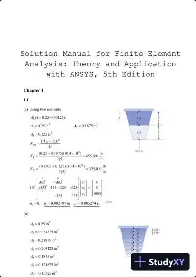 Textbook Guides
Solution Manual for Finite Element Analysis: Theory and Application with ANSYS, 5th Edition
Mechanical Engineering
426 pages53downloadsFeb 2025 Textbook Guides
Solution Manual For Modern Compressible Flow: With Historical Perspective, 3rd Edition
Mechanical Engineering
362 pages52downloadsFeb 2025 Certification Guides
Biofluid Mechanics: An Introduction to Fluid Mechanics, Macrocirculation, and Microcirculation, 3rd Edition (2021)
Mechanical Engineering
172 pages48downloadsFeb 2025 Textbook Guides
Solution Manual for Introduction to Finite Elements in Engineering, 4th Edition
Mechanical Engineering
308 pages47downloadsFeb 2025
Study this document with CramX
Once it is in your library, every tool can work from it.