

Statistics For The Behavioral Sciences, 9th Edition Solution Manual
- Statistics
- 85 pages
- Shared May 2025
Statistics For The Behavioral Sciences, 9th Edition Solution Manual provides step-by-step solutions and explanations for better comprehension.
Preview 16 of 85 pages
See the first 16 pages exactly as they appear in the document.
Page 1 Read page 1 as text
Solutions - page 280 Solutions for End - of - Chapter Problems Note: Many of the problems in the text require several stages of computation. At each stage there is an opportunity for rounding answers. Depending on the exact sequence of operations used to solve a problem, different individuals will round their answers at different times and in different ways. As a result, you or your students may obtain answers that are slightly different from those presented here. To help minimize this problem, we have tried to include the numerical values obtained at different stages of complex problems rather than presenting a single final answer.
Page 2 Page 3 Read page 3 as text
Solutions - Chapter 1 - page 281 Chapter 1: Introduction to Statistics 1. a. The population is the entire set of adolescent boys who are taking medication for depression. b. The sample is the group of 30 boys who were tested in the study. 2. A parameter is a characteristic, usually a numerical value, that describes a population. A statistic is a characteristic, usually numerical, that describes a sample. 3 Descriptive statistics are used to simplify and summarize data. Inferential statistics use sample data to make general conclusions about populations. 4. a. If treatments 1 and 2 affect individuals differently, then the scores in the first sample will be different from the scores in the second sample. b. Even if the two treatments have exactly the same effect, you do not expect the individuals in one condition to behave exactly the same as the individuals in the other treatment. The two groups will produce different scores with different means. In this case, the differences are the result of sampling error. 5. A correlational study ha s only one group of individuals and measures two (or more) different variables for each individual . Other research methods evaluating relationships between variables compare two (or more) different groups of scores. 6. The goal of an experiment is to demonstrate the existence of a cause - and - effect relationship between two variables. To accomplish the goal, an experiment must manipulate an independent variable and control other, extraneous variables. 7. The independent variable is holding a pen in your teeth versus holding the pen in your lips. The dependent variable is the rating given to each cartoon. 8. This is not an experiment because no independent variable is manipulated. They are comparing two preexisting groups of individuals. 9. a. This is a nonexperimental study. The researcher is simply observing, not manipulating, two variables. b. This is an experiment. The researcher is manipulating the type of drink and should control other variables by beginning with equivalent groups of participants. 10. a. The dependent variable is the number of colds each participant has during the winter. b. discrete c. ratio scale (zero means none)
Page 4 Read page 4 as text
Solutions - Chapter 1 - page 282 11. This is not an experiment because there is no manipulation. Instead, the study is comparing two preexisting groups (American and Canadian students). 1 2. The independent variable is the substance that is inhaled, either oxytocin or the inactive placebo. The dependent variable is how likely the people were to give their money to the trustee. 1 3. a. continuous. The variable is the amount of time and time is infinitely divisible. b. discrete. Family size consists of whole - number categories that cannot be divided. c. discrete. There are two separate and distinct categories (analog and digital). d. continuous. The variable is knowledge of statistics, which is measured with quiz scores. It could be a 5 - point quiz, a 10 - point quiz, or a 50 - point quiz, which indicates that knowledge can be divided indefinitely. 14. a. An ordinal scale provides information about the direction of difference (greater or less) between two measurements. b. An interval scale provides information about the magnitude of the difference between two measurements. c. A ratio scale provides information about the ratio of two measurements. 15. a. The independent variable is humorous versus nonhumorous. b. The independent variable is measured on a nominal scale. c. The dependent variable is the number of sentences recalled. d. The dependent variable is measured on a ratio scale. 16. Shyness is an internal attribute or characteristic that cannot be observed or measured directly. Shyness could be operationally defined by identifying and observing external behaviors associated with shyness. Or, participants could be given a questionnaire asking how they behave or feel in situations for which shyness might have an influence. 17. a. The independent variable is whether or not the motivational signs were posted, and the dependent variable is amount of use of the stairs. b. Posting versus not posting is measured on a nominal scale. 18. a. X = 12 b. X 2 = 46 c. ( X ) 2 = (12) 2 = 144 d. ( X – 1) = 8 19. a. X = 15 b. X 2 = 65 c. ( X + 1) = 20 d. ( X + 1) 2 = 100
Page 5 Read page 5 as text
Solutions - Chapter 1 - page 283 20. a. X = – 8 b. X 2 = 22 c. ( X + 4) = 12 21. a. X = 11 b. Y = 25 c. XY = 54 22. a. Σ( X + 1) b. Σ( X + 1) 2 c. (Σ X ) 2 – 3 23. a. X 2 = 30 b. ( X ) 2 = 64 c. ( X – 2) = 0 d. ( X – 2) 2 = 14
Page 6 Read page 6 as text
So lutions - Chapter 2 - page 284 Chapter 2: Frequency Distributions 1. X f ──── 10 3 9 6 8 4 7 2 6 3 5 1 4 1 ──── 2. X f p % ──────────── 9 2 0.10 10% 8 3 0.15 15% 7 5 0.25 25% 6 4 0.20 20% 5 3 0.15 15% 4 2 0.10 10% 3 1 0.05 5% ──────────── 3. a. n = 12 b. Σ X = 40 c. Σ X 2 = 148 4. a. n = 14 5. a. X f b. X f b. Σ X = 35 28 - 29 1 25 - 29 8 c. Σ X 2 = 107 26 - 27 4 20 - 24 10 24 - 25 7 15 - 19 3 22 - 23 4 10 - 14 2 20 - 21 2 5 - 9 1 18 - 19 2 16 - 17 1 14 - 15 0 12 - 13 1 10 - 11 1 8 - 9 1
Page 7 Read page 7 as text
So lutions - Chapter 2 - page 285 6. X f 60 - 64 1 55 - 59 2 50 - 54 2 45 - 49 1 Younger drivers, especially those 20 to 29 40 - 44 2 years old, tend to get more tickets. 35 - 39 3 30 - 34 3 25 - 29 5 20 - 24 8 15 - 19 3 7. a. 2 points wide and around 8 intervals b. 5 points wide and around 12 intervals or 10 points wide and around 6 intervals c. 10 points wide and around 9 intervals 8. A regular table reports the exact frequency for each category on the scale of measurement. After the categories have been grouped into class intervals, the table reports only the overall frequency for the interval but does not indicate how many scores are in each of the individual categories. 9. A bar graph leaves a space between adjacent bars and is used with data from nominal or ordinal scales. In a histogram, adjacent bars touch at the real limits. Histograms are used to display data from interval or ratio scales. 10. a. X f 10 1 9 0 8 1 7 3 6 1 5 2 4 5 3 4 2 2 1 1
Page 8 Read page 8 as text
So lutions - Chapter 2 - page 286 b. 5 │ ┌───┐ │ │ │ 4 │ ┌───┤ │ │ │ │ │ 3 │ │ │ │ ┌───┐ │ │ │ │ │ │ 2 │ ┌───┤ │ ├───┐ │ │ f │ │ │ │ │ │ │ │ 1 │ ┌───┤ │ │ │ ├───┤ ├───┐ ┌───┐ │ │ │ │ │ │ │ │ │ │ │ │ └─┴───┴───┴───┴───┴───┴───┴───┴───┴───┴───┴─── X 1 2 3 4 5 6 7 8 9 10 11 11 . 7│ 7│ 6│ ┌───┐ 6│ 5│ │ │ 5│ 4│ ┌───┤ │ 4│ f 3│ │ │ ├───┐ 3│ 2│ │ │ │ │ 2│ 1│┌───┤ │ │ ├─── ┬ ───┐ 1│ └┴───┴───┴───┴───┴───┴───┴── └ 2 3 4 5 6 7 2 3 4 5 6 7 12. a. histogram or polygon (ratio scale) b. bar graph (ordinal scale) c. bar graph (nominal scale) d. histogram or polygon (ratio scale) e. bar graph (ordinal scale)
Page 9 Read page 9 as text
So lutions - Chapter 2 - page 287 13. a. A bar graph should be used for measurements from an ordinal scale. b. 140 │ │ 120 │ │ 100 │ │ f 80 │ │ 60 │ │ 40 │ │ 20 │ │ ─────────────────────────────────── S M L XL XXL T - shirt size 14. A bar graph is appropriate for scores measured on an ordinal scale. 160 │ │ 140 │ │ 120 │ │ f 100 │ │ 80 │ │ 60 │ │ 40 │ │ ─────────────────────────────────── A B C D F Grade 15. a. ──── X f ──── 9 1 8 1 7 4 6 5 5 7 4 2 ──── b. positively skewed
Page 10 Read page 10 as text
So lutions - Chapter 2 - page 288 16. ──── X f ──── 8 2 7 4 The distribution in negatively skewed. 6 5 5 3 4 2 3 1 2 2 1 1 ──── 17. a. ───── X f ───── 10 1 9 2 8 2 7 2 6 4 5 3 4 2 3 2 2 1 ───── b. │ 4 │ │ 3 │ f │ 2 │ │ 1 │ │ └──────────────────────────────── ─ X 1 2 3 4 5 6 7 8 9 10 c. It is a fairly symmetrical distribution centered at X = 6. The scores are scattered across the scale.
Page 11 Read page 11 as text
So lutions - Chapter 2 - page 289 18. 6 5 ○ ○ - - - ○ Unhappy f 4 —— Happy 3 ○ 2 ○ ○ 1 ○ ○ ———————————————————————— 1 2 3 4 5 6 7 8 9 10 Number of Friends Yes, it appears that the happy people tend to have more friends than the unhappy people do. 19. ────────────── X f cf c % ────────────── 7 2 25 100 6 3 23 92 5 6 20 80 4 9 14 56 3 4 5 20 2 1 1 4 ────────────── a. T he percentile rank for X = 2.5 is 4% b. T he percentile rank for X = 6.5 is 92% c. The 20 th percentile is X = 3 .5. d. The 80 th percentile is X = 5.5. 20. ────────────── X f cf c % ────────────── 50 - 59 1 20 100 40 - 49 3 19 95 30 - 39 6 16 80 20 - 2 9 5 10 50 10 - 19 3 5 25 0 - 9 2 2 10 ──────────────
Page 12 Read page 12 as text
So lutions - Chapter 2 - page 290 a. T he percentile r ank for X = 9.5 is 10% b. T he percentile rank for X = 3 9 .5 is 80% c. The 25 th percentile is X = 19.5. d. The 50 th percentile is X = 29.5. 21. ────────────── X f cf c % ────────────── 10 2 50 100 9 5 48 96 8 8 43 86 7 15 35 70 6 10 20 40 5 6 10 20 4 4 4 8 ────────────── a. T he percentile rank for X = 6 is 30%. b. T he percentile rank for X = 9 is 91% c. T he 25 th percentile is X = 5.75. d. T he 90 th percentile is X = 8.9. 22. a. T he percentile rank for X = 15 is 17.5%. b. T he percentile rank for X = 18 is 77.5%. c . The 15 th percentile is X = 14.75. d. The 90 th percentile is X = 19. 23. a. T he percentile rank for X = 5 is 8%. b. T he percentile rank for X = 12 is 85%. c . The 25 th percentile is X = 7. d. The 70 th percentile is X = 10. 24. a. The 30 th percentile is X = 72. b. The 88 th percentile is X = 93.5. c. The percentile rank for X = 77 is 40%. d. The percentile rank for X = 90 is 81%. 25. 1│796 2│0841292035826 3│094862 4│543 5│3681 6│4
Page 13 Read page 13 as text
So lutions - Chapter 2 - page 291 26. a. 4 b. 72, 71, 78, and 74 c. 2 d. 46 an d 40 27 . 2 │ 80472 3 │ 49069 4 │ 543976 5 │ 4319382 6 │ 5505 7 │ 24 8 │ 1
Page 14 Read page 14 as text
Solutions - Chapter 3 - page 292 Chapter 3: Central Tendency 1. The purpose of central tendency is to identify a single score that serves as the best representative for an entire distribution, usually a score from the center of the distribution. 2. No single method for computing a measure of central tendency works well in all situations. With three different methods, however, at least one usually works well 3. The mean is 29/10 = 2.9, the median is 2.5, and the mode is 2. 4. For this sample, the mean is 94/12 = 7.83, the median is 8, and the mode is 8. 5. The mean is 69/12 = 5.75, the median is 6, and the mode is 7. 6. The mean is 107/15 = 7.13, the median is 7, and the mode is 6. 7. a. Median = 2.83 (2.5 + 0.33) b. Median = 3 8. X = 63. 9. N = 25 10. The original sample has n = 8 and Σ X = 80. The new sample has n = 9 and Σ X = 81. The new mean is M = 9. 11. The original sample has n = 5 and Σ X = 60. The new sample has n = 4 and Σ X = 52. The new mean is M = 13. 12. With the new score, n = 12, Σ X = 60, and M = 5. 13. After the s core is removed, n = 8 , Σ X = 88, and M = 11. 14. After the score is changed, N = 20, Σ X = 320, and μ = 16. 15. After the score is changed, n = 7, Σ X = 49, and M = 7. 16. The original sample has n = 7 and Σ X = 35. The new sample has n = 8 and Σ X = 48 . The new score must be X = 13. 17. The original sample has n = 16 and Σ X = 320. The new sample has n = 15 and Σ X = 285. The score that was removed must be X = 35.
Page 15 Read page 15 as text
Solutions - Chapter 3 - page 293 18. a. The new mean is M = 6. b. The new mean is (12 + 56)/10 = 6.8. c. The new mean is (28 + 24)/10 = 5.2. 19. a. The new mean is 75/10 = 7.5. b. The new mean is (20 + 60)/10 = 8 c. The new mean is (30 + 40)/10 = 7 20. With a skewed distribution, the extreme scores in the tail can displace the mean out toward the tail. The result is that the mean is often not a very representative value. 21. The median is used instead of the mean when there is a skewed distribution (a few extreme scores), an open - ended distribution, undetermined scores, or an ordinal scale. 22. a. With one extreme score, the median would be better than the mean. b. With a nominal scale, the mode is the only option. c. With numerical scores, the mean is usually best. 23. a. Mode = 2 b. Median = 2 c. You cannot find the total number of fast - food visits (Σ X ) for this sample. 24. a. 5 │ │ 4 │ ┌───┐ │ │ │ 3 │ ┌───┬───┤ │ │ │ │ │ │ 2 │ ┌───┐ │ │ │ ├───┐ ┌───┐ f │ │ │ │ │ │ │ │ │ │ 1 │ ┌───┬───┤ ├───┤ │ │ │ ├───┤ │ │ │ │ │ │ │ │ │ │ │ │ │ └─┴───┴───┴───┴───┴───┴───┴───┴───┴───┴───┴─ X 1 0 +1 +2 +3 +4 +5 +6 +7 +8 Weight change (in pounds) during the first semester of freshman year b. The mean difference in weight is M = 79/20 = +3.95 pounds. On average, the students gained 3.95 points duri ng the semester. c. Yes, nearly all the students showed some weight gain. 25. a. For weekdays M = 0.99 inches and for weekend days is M = 1.67 inches. b. There does appear to be more rain on weekend days than there is on weekdays.
Page 16 Read page 16 as text
Solutions - Chapter 4 - page 294 Chapter 4: Variability 1. a. SS is the sum of squared deviation scores. b. Variance is the mean squared deviation. c. Standard deviation is the square root of the variance. It provides a measure of the standard distance from the mean. 2. SS cannot be less than zero because it is computed by adding squared deviations. Squared deviations are always greater than or equal to zero. 3. Standard deviation and variance are measures of distance and are always greater than or equal to zero. 4. A standard deviation of zero indicates there is no variability. In this case, all of the scores in the sample have exactly the same value. 5. Without some correction, the sample variance underestimates the variance for the population. Changing the formula for sample variance (using n – 1 instead of N ) is the necessary correction. 6. a. No. X = 70 is 10 points away from the mean, only ½ of the standard deviation. b. Yes. With s = 5, 10 points is equal to a distance of 2 standard deviations . 7. a. s = 2 is better (you are above the mean by 3 standard deviations). b. s = 10 is better (you are below the mean by less than half a standard deviation). 8. a. The mean is μ = 35 and the standard deviation is still σ = 5. b. The new mean is μ = 90 and the new standard deviation is σ = 15. 9. a. The original mean is M = 80 and the standard deviation is s = 8. b. The original mean is M = 12 and the standard deviation is s = 3. 10. The mean is M = 86 and the standard deviation is s = 3. 11. a. The range is either 11 or 12, and the standard deviation is σ = 4. b. After adding 2 points to each score, the range is still either 11 or 12, and the standard deviation is still σ = 4. Adding a constant to every score does not affe ct measures of variability. 12. a. The definitional formula is easy to use when the mean is a whole number and there are relatively few scores. b. The computational formula is preferred when the mean is not a whole number.
69 more pages in the full document
Unlock it once and it stays in your library, ready to chat with or turn into flashcards.
Unlock the full documentMore Statistics study materials
See all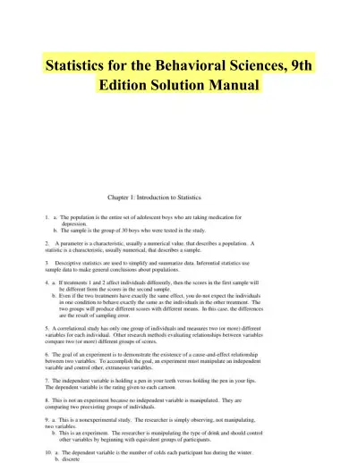 Textbook Guides
Statistics for the Behavioral Sciences, 9th Edition Solution Manual
Statistics
85 pagesMay 2025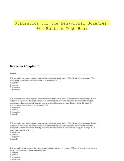 Exam Guides
Statistics for the Behavioral Sciences, 9th Edition Test Bank
Statistics
491 pagesMay 2025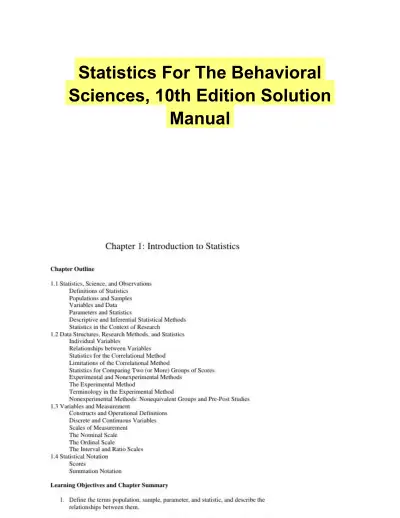 Textbook Guides
Statistics For The Behavioral Sciences, 10th Edition Solution Manual
Statistics
94 pagesMay 2025 Exam Guides
Test Bank for Biostatistics for the Biological and Health Sciences , 2nd Edition
Statistics
182 pages161downloadsFeb 2025 Exam Guides
Elementary Statistics, 13th Edition Test Bank
Statistics
239 pages160downloadsFeb 2025 Textbook Guides
Solution Manual For Statistics for Managers Using Microsoft Excel, 7th Edition
Statistics
1418 pages158downloadsFeb 2025 Textbook Guides
Statistics for Managers Using Microsoft Excel 8th Edition Solution Manual
Statistics
1343 pages156downloadsFeb 2025 Textbook Guides
Essentials of Social Statistics for a Diverse Society Second Edition Solution Manual
Statistics
137 pages135downloadsFeb 2025
Study this document with CramX
Once it is in your library, every tool can work from it.