Solution Manual for Digital Control System Analysis Design, 4th Edition

Preview (16 of 279 Pages)

100%

Solution Manual for Digital Control System Analysis Design, 4th Edition - Page 1 preview image

Loading page ...

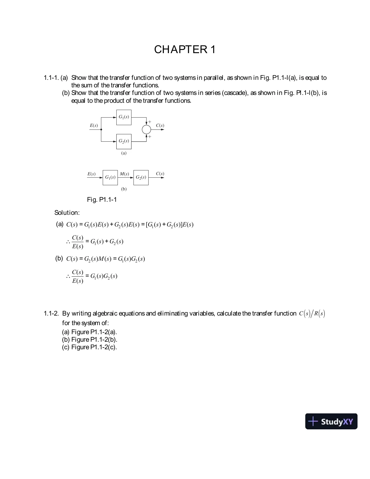
CHAPTER 11.1-1.(a) Show that the transfer function of two systems in parallel, as shown in Fig. P1.1-l(a), is equal tothe sum of the transfer functions.(b) Show that the transfer function of two systems in series (cascade), as shown in Fig. Pl.1-l(b), isequal to the product of the transfer functions.G1(s)E(s)C(s)G1(s)G2(s)(a)(b)E(s)M(s)G2(s)C(s)++Fig. P1.1-1Solution:(a)1212( )( )( )( )( )[( )( )]( )C sG s E sGs E sG sGsE s=+=+12( )( )( )( )C sGsGsE s∴=+(b)212( )( )( )( )( )C sGs M sGs Gs==12( )( )( )( )∴=C sGs GsE s1.1-2.By writing algebraic equations and eliminating variables, calculate the transfer functionC s( )R s( )for the system of:(a) Figure P1.1-2(a).(b) Figure P1.1-2(b).(c) Figure P1.1-2(c).

Solution Manual for Digital Control System Analysis Design, 4th Edition - Page 2 preview image

Loading page ...

Solution Manual for Digital Control System Analysis Design, 4th Edition - Page 3 preview image

Loading page ...

(a)(b)E(s)Gc(s)H(s)M(s)R(s)Gp(s)C(s)-+(c)G1(s)G2(s)E(s)R(s)++-+M(s)G3(s)C(s)H(s)E(s)G1(s)H2(s)H1(s)M(s)R(s)G2(s)C(s)-+++Fig. P1.1-2Solution:(a)( )( )( )( )( )( )( )( )[( )( )( )]pcpcpC sGs M sGs Gs E sGs GsR sH s C s===−[1( )( )( )]( )( )( )( )cpcpGs Gs H sC sGs Gs R s+=( )( )( )( )1( )( )( )cpcpGs GsC sR sGs Gs H s∴=+(b)C(s)=G3(s)M(s)=G3(s)[G1(s)E(s)+G2(s)R(s)]3123( )( )[( )( )( )]( )( )( )Gs G sR sH s C sGs Gs R s=−+13123[1( )( )( )]( )[( )( )]( )( )G s Gs H s C sG sGs Gs R s+=+∴C(s)R(s)=[G1(s)+G2(s)]G3(s)1+G1(s)G3(s)H(s)(c)2121221( )( )( )( )( )( )( )( )[( )( )( )( )( )]===−−C sGs M sG s Gs E sG s GsR sHs M sHs C s2and( )( )( )=M sC sGs1221211221( )( )G G HG G HC sG G R sG⎡⎤∴++=⎢⎥⎣⎦∴C(s)R(s)=G1(s)G2(s)1+G1(s)H2(s)+G1(s)G2(s)H1(s)

Solution Manual for Digital Control System Analysis Design, 4th Edition - Page 4 preview image

Loading page ...

1.1-3.Use Mason’s gain formula of Appendix II to verify the results of Problem 1.1-2 for the system of:(a) Figure P1.1-2(a).(b) Figure P1.1-2(b).(c) Figure P1.1-2(c).Solution:(a)( )( )( )( )1( )( )( )cpcpGs GsC sR sGs Gs H s=+(b)132313( )( )( )( )( )( )1( )( )( )Gs GsGs GsC sR sGs Gs H s+=+(c)1212121( )( )( )( )1( )( )( )( )( )Gs GsC sR sGs HsGs Gs Hs=++1.1-4.A feedback control system is illustrated in Fig. P1.1-4. The plant transfer function is given byGps( ) =50.2s+1Gc(s)Gp(s)CompensatorH(s)R(s)E(s)M(s)C(s)SensorPlant+-Fig. P1.1-4(a) Write the differential equation of the plant. This equation relatesc t( )andm t( ).(b) Modify the equation of part (a) to yield the system differential equation; this equation relatesc t( )andr t( ). The compensator and sensor transfer functions are given byGcs( ) =10,H s( ) =1(c) Derive the system transfer function from the results of part (b).(d) It is shown in Problem 1.1-2(a) that the closed-loop transfer function of the system of Fig.P1.1-4 is given byC s( )R s( ) =Gcs( )Gps( )1+Gcs( )GPs( )H s( )Use this relationship to verify the results of part (c).(e) Recall that the transfer-function pole terms+a()yields a time constantτ=1a, whereaisreal. Find the time constants for both the open-loop and closed-loop systems.Solution:(a)( )525( )(5)( )25( )( )0.215===⇒+=++pC sGssC sM sM sss

Solution Manual for Digital Control System Analysis Design, 4th Edition - Page 5 preview image

Loading page ...

( )5 ( )25( )dc tc tm tdt∴+=(b)m(t)=10e(t)=10[r(t)−c(t)]∴!c(t)+5c(t)=250[r(t)−c(t)]∴!c(t)+255c(t)=250r(t)(c)5( )255( )250( )C sC sR s+=( )250( )255C sR ss∴=+(d)C(s)R(s)=(10)25s+51+(10)25s+5 (1)=250s+255(e) open-loop:0.2sτ=closed-loop:τ1 2550.00392s==1.1-5.Repeat Problem 1.1-4 with the transfer functionsGcs( ) =2,Gps( ) =3s+8s2+2s+2,H s( ) =1For part (e), recall that the transfer-function underdamped pole term[s+a()2+b2]yields a timeconstant,τ=1a.Solution:(a)2( )38( )( )22C ssG sM sss+==++∴(s2+2s+2)C(s)=(3s+8)M(s)!!c(t)+2!c(t)+2c(t)=3!m(t)+8m(t)(b)( )2 ( )2[ ( )( )]m te tr tc t==−∴!!c(t)+2!c(t)+2c(t)=6[!r(t)−!c(t)]+16[r(t)−c(t)]∴!!c(t)+8!c(t)+18c(t)=6!r(t)+16r(t)(c)2(818)( )(616)( )ssC ssR s++=+2( )616( )818C ssR sss+∴=++(d)22238(2)( )6162238( )8181(2)(1)22sC sssssR sssss++++==++++++

Solution Manual for Digital Control System Analysis Design, 4th Edition - Page 6 preview image

Loading page ...

(e) open-loop:2221sssj++⇒=−±∴term=A1ε−tcos(t+θ1);τ=1 1=1sclosed-loop:281842sssj++⇒=−±∴term=A2ε−4tcos(2t+θ2);τ=1 4=0.25s1.1-6.Repeat Problem 1.1-4 with the transfer functionsGcs( ) =2,Gps( ) =5s2+2s+2,H s( ) =3s+1Solution:(a)22( )5( )(22)( )5( )( )22C sG sssC sM sM sss==⇒++=++∴!!c(t)+2!c(t)+2c(t)=5m(t)(b)( )( )(31)( )E sR ssC s=−+∴e(t)=r(t)−3!c(t)−c(t)∴!!c(t)+2!c(t)+2c(t)=5[2e(t)]=10r(t)−30!c(t)−10c(t)∴!!c(t)+32!c(t)+12c(t)=10r(t)(c)2(3212)( )10( )ssC sR s++=2( )10( )3212C sR sss∴=++(d)2225(2)( )10225( )32121(2)(31)22C sssR ssssss++==++++++(e)open-loop:τ=1s, from Problem 1.1-5(e)closed-loop: poles1624431.62,0.38=−±=−−121 31.620.0316 ;1 0.382.63ss∴τ==τ==1.4-1.The satellite of Section 1.4 is connected in the closed-loop control system shown in Fig. P1.4-1.The torque is directly proportional to the error signal.

Solution Manual for Digital Control System Analysis Design, 4th Edition - Page 7 preview image

Loading page ...

ThrustersThrustersw(t)(a)(b)KAmplifiers andthrustersH(s)=1®c(s)E(s)ErrorT(s)Torque®(s)SensorSatellite+-1Js2Fig. P1.4-1(a) Derive the transfer functionΘ(s) /Θcs( ), whereθt( ) =L−1Θ(s)⎡⎣⎢⎤⎦⎥is the commanded attitudeangle.(b) The state equations for the satellite are derived in Section 1.4. Modify these equations to modelthe closed-loop system of Fig. P1.4-1.Solution:(a)2221( )( )( )[( )( )]cKKsT sE sssJsJsJsΘ===Θ− Θ∴1+KJs2⎡⎣⎢⎤⎦⎥ Θ(s)=KJs2Θc(s)222( )( )1csK JsK JKssK JJsΘ∴==Θ++(b)(1−4):x1=0; (1−5):x2=!θ=!x1∴!x2(t)=!!θ(t)=1Jτ(t)=KJ e(t)=KJ[θc(t)− θ(t)]1[θ( )( )]cKtxtJ=−

Solution Manual for Digital Control System Analysis Design, 4th Edition - Page 8 preview image

Loading page ...

∴!x1(t)!x2(t)⎡⎣⎢⎢⎤⎦⎥⎥=01K J0⎡⎣⎢⎢⎤⎦⎥⎥x1(t)x2(t)⎡⎣⎢⎢⎤⎦⎥⎥+0K J⎡⎣⎢⎢⎤⎦⎥⎥"c(t)( )[10] ( )y tx t=1.4-2.(a) In the system of Problem 1.4-1,J= 0.4andK= 14.4, in appropriate units. The attitude of thesatellite is initially at 0°. Att= 0, the attitude is commanded to 20°; that is, a 20° step is appliedatt= 0. Find the responseθ(t).(b) Repeat part (a), with the initial conditionsθ(0) = 10° and!θ0( ) =30°/s. Note that we haveassumed that the units of time for the system is seconds.(c) Verify the solution in part (b) by first checking the initial conditions and then substituting thesolution into the system differential equation.Solution:(a)From Problem 1.4-1,Θ(s)Θc(s)=36s2+36∴ Θ(s)=36s2+36×20s=720s(s2+36)=20s+as+bs2+3622220720;0,20(36)sasbsbas s+++=∴==−+22020( )( )20[1cos 6 ],036sstttss−∴Θ=+⇒ Θ=−≥+(b)From (a),!!θ(t)+36θ(t)=36θc(t)∴(s2+36)Θ(s)−sθ(0)−!θ(0)=36Θc(s)∴ Θ(s)=36s2+36Θc(s)+10ss2+36+30s2+3622220201030363636ssssss=−+++++222010303636ssss=−+++∴ θ(t)=20−10cos6t+5sin 6t,t≥0(c)θ(0)=20−10=10°!θ(t)=60sin 6t+30cos6t⇒!θ(0)=30°sFrom (b),!!θ+36θ=720∴360cos6t−180sin 6t+720−360cos6t+180sin 6t=720720720∴=

Solution Manual for Digital Control System Analysis Design, 4th Edition - Page 9 preview image

Loading page ...

1.4-3.The input to the satellite system of Fig. P1.4-1 is a step functionθct( ) =5u t( )in degrees. As aresult, the satellite angleθt( )varies sinusoidally at a frequency of 10 cycles per minute. Find theamplifier gainKand the moment of inertiaJfor the system, assuming that the units of time in thesystem differential equation are seconds.Solution:From Problem 1.4-1,Θ(s)=K Js2+K J×5s=a25(s2+a2)s,a2=K J2255( )ssssa∴ Θ=−+∴ θ(t)=5−5cosat,t≥01min11rad10 cy mincy s2πs6066as⎛⎞×=⇒=⎜⎟⎝⎠∴a=π3=K J,∴KandJcannot be determined without additional data.1.4-4.The satellite control system of Fig. P1.4-1 is not usable, since the response to any excitationincludes an undamped sinusoid. The usual compensation for this system involves measuring theangular velocitydθt( )dt. The feedback signal is then a linear sum of the position signalθt( )andthe velocity signaldθt( )dt.This system is depicted in Fig. P1.4-4, and is said to haveratefeedback.SatelliteKT®®Kv1s1JsR(s)E+-++Fig. P1.4-4(a) Derive the transfer functionΘ(s) /Θc(s)for this system.(b) The state equations for the satellite are derived in Section 1.4. Modify these equations to modelthe closed-loop system of Fig. P1.4-4.(c) The state equations in part (b) can be expressed asxt( ) =Axt( ) +Bθct( )

Solution Manual for Digital Control System Analysis Design, 4th Edition - Page 10 preview image

Loading page ...

The system characteristic equation issI−A=0Show thatsI−Ain part (b) is equal to the transfer function denominator in part (a).Solution:(a)Θ(s)=1s!Θ(s)=1Js2T(s)=KTs2[Θc(s)−Kv!Θ(s)− Θ(s)]!Θ(s)=sΘ(s)∴ Θ(s)=KJs2[Θc(s)−(Kvs+1)Θ(s)]∴ Θ(s)Θc(s)=KJs2+KKvs+K=K Js2+KKvJs+KJ(b)x1(t)=θ(t);x2(t)=!x1(t)=θ(t)∴!x2(t)=!!θ(t)=1Jτ(t)=KJ[θc(t)−Kvx2(t)−x1(t)]∴!x(t)=01−K J−KKvJ⎡⎣⎢⎢⎤⎦⎥⎥x(t)+0K J⎡⎣⎢⎢⎤⎦⎥⎥θc(t)θ(t)=10⎡⎣⎤⎦x(t)(c)| sI−A|=s−1K JS+KKvJ=s2+KKvJs+KJ1.5-1.The antenna positioning system described in Section 1.5 is shown in Fig. P1.5–1. In this problemwe consider the yaw angle control system, whereθt( )is the yaw angle. Suppose that the gain ofthe power amplifier is 10 V/V, and that the gear ratio and the angle sensor (the shaft encoder andthe data hold) are such thatvot( ) =0.04θt( )where the units ofvot( )are volts and ofθt( )are degrees. Lete t( )be the input voltage to themotor; the transfer function of the motor pedestal is given asΘs( )E s( ) =20s s+6()

Solution Manual for Digital Control System Analysis Design, 4th Edition - Page 11 preview image

Loading page ...

(a)(b)PoweramplifierMotor/antennaVi(s)Vo(s)E(s)SensorKInputgain+-®1(s)®(s)Voltageproportionalto desiredangleVoltageproportionalto angleMotorshaftTop view of pedestalDifferenceamplifierPoweramplifierMotorvoltagee(t)MotorGearsAntennaSide viewof pedestalShaftencoderBinarycodeDataholdErrorvivi-voh(t)w(t)voFig. P1.5-1(a) With the system open loop [vot( )is always zero], a unit step function of voltage is applied tothe motorE s( ) =1s⎡⎣⎢⎤⎦⎥. Consider only thesteady-state response.Find the output angleθt( )indegrees, and the angular velocity of the antenna pedestal,θt( ), in both degrees per second andrpm.(b) The system block diagram is given in Fig. P1.5-1(b), with the angle signals shown in degreesand the voltages in volts. Add the required gains and the transfer functions to this blockdiagram.(c) Make the changes necessary in the gains in part (b) such that the units ofθt( )are radians.(d) A step input ofθit( ) =10°is applied at the system input att=0. Find the responseθt( ).(e) The response in part (d) reaches steady state in approximately how many seconds?Solution:(a)Θ(s)=20s2(s+6)=3.33s2+ks+5 9s+6

Solution Manual for Digital Control System Analysis Design, 4th Edition - Page 12 preview image

Loading page ...

k=dds20s+6⎡⎣⎢⎤⎦⎥s=0=−20(s+6)2s=0=−59∴ θss(t)=3.33t−59⎛⎝⎜⎞⎠⎟in degrees!θss(t)=3.33 deg / s∴3.33ds×60s1 min×1rcv360°=59rpm(b)+-∫i(s)∫(s)0.04degVi(s)GiKiH0.041020s(s+6)E(s)VO(s)(c)1 degree=π180 rad+-∫i(s)∫(s)0.04radVi(s)1020s(s+6)0.04180rr180E(s)VO(s)365rr9+-∫i(s)∫(s)0.04Vi(s)10s(s+6)E(s)VO(s)(d)220(0.04)(10)( )8(6)20( )681(0.04)(10)(6)Θ+==Θ++++iss sssss s810102010( )(2)(4)24−Θ=×=++++++sssssss24θ( )102010,0tttet−−∴=−ε+≥(e)121112,0.5,0.25,4(0.5)24tssts− τε⇒=τ=τ==∴≈=τ

Solution Manual for Digital Control System Analysis Design, 4th Edition - Page 13 preview image

Loading page ...

1.5-2.The state-variable model of a servomotor is given in Section 1.5. Expand these state equations tomodel the antenna pointing system of Problem 1.5-1(b).Solution:From Eqn. (1-15)Gp(s)=KTJRass+BRa+KTKbJRa⎛⎝⎜⎞⎠⎟=20s(s+6) ,∴KTJRa=20;BRa+KTKbJRa=6From Eqn (1−16),x1=θ;x2=!θ=!x1From Eqn (1−17),!x2(t)=!!θ(t)=−6x2(t)+20e(t)=−6x2(t)+20(10[0.04θi(t)−0.04θ(t)])=−6x2(t)+8θi(t)−8x1(t)∴!x(t)=01−8−6⎡⎣⎢⎤⎦⎥x(t)+08⎡⎣⎢⎤⎦⎥ θi(t)θ(t)=10⎡⎣⎤⎦x(t)1.5-3.(a) Find the transfer functionΘs( )/Θis( )for the antenna pointing system of Problem 1.5-1(b).This transfer function yields the angleθt( )in degrees.(b) Modify the transfer function in part (a) such that use of the modified transfer function yieldsθt( )in radians.(c) Verify the results of part (b) using the block diagram of Problem 1.5-1(b).Solution:(a)From Problem 1.5-1(d),Θ(s)Θi(s)=8s2+6s+8(b)1 deg =π180()rad∴ Θ(s)Θi(s)=8s2+6s+8×π180=2π45s2+6s+8(c)Θ(s)Θi(s)=KiG1G21+G1G2H=125⎛⎝⎜⎞⎠⎟(10)π9s(s+6)⎛⎝⎜⎞⎠⎟1+(10)π9()s(s+6)365π⎛⎝⎜⎞⎠⎟=2π45s2+6s+8

Solution Manual for Digital Control System Analysis Design, 4th Edition - Page 14 preview image

Loading page ...

1.5-4.Shown in Fig. P1.5-4 is the block diagram of one joint of a robot arm. This system is described inSection 1.5. The inputM s( )is the controlling signal,Eas( )is the servomotor input voltage,Θms( )is the motor shaft angle, and the outputΘas( )is the angle of the arm. The inductance of thearmature of the servomotor has been neglected such that the servomotor transfer function is secondorder. The servomotor transfer function includes the inertia of both the gears and the robot arm.Derive the transfer functionsΘas( )/M(s)andΘa(s) /Eas( ).PoweramplifierServomotorGearsMKEa®a®m1s11002000.5s+1Fig. P1.5-4Solution:Θa(s)=1100Θm(s)1100s!Θm(s)=2s(0.5s+1)Ea(s)=2Ks(0.5s+1)M(s)∴ Θa(s)M(s)=2Ks(0.5s+1) ;Θa(s)Ea(s)=2s(0.5s+1)1.5-5.Consider the robot arm depicted in Fig. P1.5-4.(a) Suppose that the units ofeat( )are volts, that the units of bothθmt( )andθat( )are degrees, andthat the units of time are seconds. If the servomotor is rated at 24 V [the voltageeat( )shouldbe less than or equal to 24 V], find the rated rpm of the motor (the motor rpm, in steady state,with 24 V applied).(b) Find the maximum rate of movement of the robot arm, in degrees per second, with a stepvoltage ofeat( ) =24u t( )volts applied.(c) Assume thateat( )is a step function of 24 V. Give the time required for the arm to be movingat 99 percent of the maximum rate of movement found in part (b).(d) Suppose that the inputm t( )is constrained by system hardware to be less than or equal to 10 Vin magnitude. What value would you choose for the gainK.Why?Solution:(a)!Θa(s)=20.5s+1×24s=48s(0.5s+2)=96s(s+2)=k1s+k2s+2=48s−48s+2⇒!θa(t)=48−48ε−2t,t≥0∴!θass(t)=48°s×60s1min×1rev360° =8rpm

Solution Manual for Digital Control System Analysis Design, 4th Edition - Page 15 preview image

Loading page ...

∴!θmss(t)=100!θa(t)=800 rpm(b)From (a),!θa(t)=48°s(c)From (a),!θa(t)=48(1− ε−2t),t≥0∴ τ=0.5sε−2t1=0.01⇒2t1=4.60⇒t1=2.30s(d)K=2.4⇒ea(t)=24V,rated voltage1.6-1.A thermal test chamber is illustrated in Fig. P1.6-1(a). This chamber, which is a large room, isused to test large devices under various thermal stresses. The chamber is heated with steam, whichis controlled by an electrically activated valve. The temperature of the chamber is measured by asensor based on a thermistor, which is a semiconductor resistor whose resistance varies withtemperature. Opening the door into the chamber affects the chamber temperature and thus must beconsidered as a disturbance.A simplified model of the test chamber is shown in Fig. P1.6-1(b), with the units of time inminutes. The control input is the voltagee t( ), which controls the valve in the steam line, asshown. For the disturbanced t( ), a unit step function is used to model the opening of the door.With the door closed,d t( ) =0.(a)(b)Chamber0.04SensorTemperature,5CDisturbanced(t)c(t)2s+0.52.5s+0.5Voltagee(t)Voltage+-To sensorcircuitsDoorRTThermalchamberThermistorValveSteamlineVoltagee(t)

Solution Manual for Digital Control System Analysis Design, 4th Edition - Page 16 preview image

Loading page ...

Fig. P1.6-1(a) Find the time constant of the chamber.(b) With the controlling voltagee t( ) =5u t( )and the chamber door closed, find and plot thechamber temperaturec t( ).In addition, give the steady-state temperature.(c) A tacit assumption in part (a) is an initial chamber temperature of zero degrees Celsius. Repeatpart (b), assuming that the initial chamber temperature isc0( ) =25°C.(d) Two minutes after the application of the voltage in part (c), the door is opened, and it remainsopen. Add the effects of this disturbance to the plot of part (c).(e) The door in part (d) remains open for 12 min. and is then closed. Add the effects of thisdisturbance to the plot of part (d).Solution:(a)2( );2 min0.511τ===∴ τ=+τ++τKKG ssss(b)252020( )0.50.5C sssss−=×=+++0.5( )20(1),0tc tt−∴=− ε≥( )20 Cssct=°C(t)t, min80200(c)( )2( )0.5C sE ss=+∴!c(t)+0.5c(t)=2e(t)( )(0)0.5( )2( )sC scC sE s−+=∴C(s)=2E(s)s+0.5+c(0)s+0.5⇒c(t)=20(1− ε−0.5t)from (b)!"##$##+25e−0.5t∴c(t)=20+5ε−0.5t,t≥0C(t)t, min820020025(d)Disturbance response:2.5155( )·0.50.5dCsssss−−==+++

Preview Mode

This document has 279 pages. Sign in to access the full document!

Report

Study Now!

Document Details

Related Documents

Solution Manual For Digital Control System Analysis And Design, 3rd Edition

HW4_Solution

Lab 9 Energy Skate Park

Common Electric Meters Used in the Industry

Experiment #17 DC Circuits Colin McCormick

Student Exploration Circuit Builder Build and Test

IS 3413 M03 Lab Signal Coding

Computed and digital radiography notes

How to Repair a Broken HDMI Port-A Step-by-Step Gu

Flip-Flop Timing Parameters and Circuit Behavior Analysis

Company

Explore

Study Tools