

Differential Equations - Applying Differential Equations
- Mathematics
- Texas A&M University
- 35 pages
- Shared March 2026
Preview 10 of 35 pages
See the first 10 pages exactly as they appear in the document.
Page 1 Read page 1 as text
Study Guide Differential Equations – Applying Differential Equations 1. Applications of First ‐ Order Equations First - order differential equations show up in many real - world problems — from geometry and physics to chemistry and biology. In this chapter, we explore several important applications and learn how to model and solve them. 1.1 Orthogonal Trajectories What does “orthogonal” mean? • Orthogonal means perpendicular . • A trajectory is a path or curve. So, orthogonal trajectories are two families of curves that intersect each other at right angles (90°). 1.2 How do we know two curves are perpendicular? At any point where two curves intersect: • Their slopes must be negative reciprocals of each other. • If one slope is ( m ) , the other must be ( - 1/m). Since the slope of a curve is given by its derivative, two families of curves are orthogonal wherever they intersect if: Example 1: Electric Field Lines and Equipotentials
Page 2 Read page 2 as text
Study Guide Figure 1 Electric field lines from a positive point charge spread outward in straight lines from the charge. Step 1: Describe the electric field lines If the charge is placed at the origin, the electric field lines form the family: Different values of ( c ) give different straight lines through the origin. Step 2: Find the slope of the family Differentiate: From ( y = cx ) , we get: So the slope becomes:
Page 3 Read page 3 as text
Study Guide Step 3: Find the orthogonal trajectories Orthogonal trajectories must have slopes that are negative reciprocals : This equation is separable. Step 4: Solve the differential equation Integrate both sides: Rewriting: Figure 2 Final Result The orthogonal trajectories are circles centered at the origin .
Page 4 Read page 4 as text
Study Guide Interpretation: • Electric field lines are straight rays. • Equipotential lines are concentric circles. • These always intersect at right angles. Example 2: Orthogonal Trajectories of a Family of Circles Figure 3 We are given the family: These are circles tangent to the x - axis at the origin . Step 1: Differentiate implicitly Expand and differentiate:
Page 5 Read page 5 as text
Study Guide Differentiate: Solve for (dy/dx ) : Step 2: Eliminate the parameter ( c ) From the original equation: Substitute into the slope expression: Step 3: Find the orthogonal trajectories Take the negative reciprocal: This leads to the differential equation: Step 4: Solve using an integrating factor The equation is not exact, but an integrating factor ( \ mu = x^{ - 2} ) makes it exact.
Page 6 Read page 6 as text
Study Guide After integrating: Figure 4 Final Result The orthogonal trajectories are also circles tangent to the x - axis at the origin . 1.3 Radioactive Decay Some atomic nuclei are unstable and decay over time. The rate of decay depends on how much of the substance is present. The basic model Let ( x(t) ) be the amount of radioactive material at time ( t ) : Solution of the equation This separable equation gives: This curve is called an exponential decay curve .
Page 7 Read page 7 as text
Study Guide Half - Life The half - life ( T 1/2 ) is the time it takes for half of the substance to decay. From the formula: A shorter half - life means faster decay. 1.4 Radiocarbon Dating • Carbon - 14 ( 14 C) is radioactive. • Living organisms constantly absorb it. • After death, absorption stops and decay begins. Since the half - life of ( 14 C ) is 5730 years , measuring how much remains allows scientists to estimate age. Example 3: Dating a Bone A bone contains 20% of its original ( 14 C). Using: Solve for ( t ) : 1.5 Newton’s Law of Cooling When a hot object is placed in a cooler environment, its temperature decreases over time.
Page 8 Read page 8 as text
Study Guide The law states: where: • ( T ) = object temperature • ( T s ) = surrounding temperature • ( k > 0 ) Solution Solving gives: Example 4: Cooling Coffee (Newton’s Law of Cooling) A cup of coffee at 190°F is placed in a room where the temperature is 70°F . After 5 minutes , the coffee cools to 160°F . Question: How many more minutes will it take for the coffee to cool to 130°F ? Step 1: Use Newton’s Law of Cooling Newton’s Law of Cooling says that the rate at which an object cools is proportional to the difference between its temperature and the surrounding temperature. The temperature model is:
Page 9 Read page 9 as text
Study Guide where: • ( T s = 70°F ) (room temperature) • ( c ) and ( k ) are constants • ( t ) is time in minutes So we start with: Step 2: Find the constant ( c ) We know the initial temperature is 190°F: Substitute: Now the temperature model becomes: Step 3: Find the cooling constant ( k ) We are told that after 5 minutes, the temperature is 160°F:
Page 10 Read page 10 as text
Study Guide Solve step by step: Step 4: Write the final temperature formula Substitute ( k ) into the equation: Step 5: Find when the coffee reaches 130°F Set ( T(t) = 130 ) : Solve: Final Answer It takes 12 minutes total for the coffee to cool from 190°F to 130°F. Since the coffee already cooled for 5 minutes , the additional time required is:
25 more pages in the full document
Unlock it once and it stays in your library, ready to chat with or turn into flashcards.
Unlock the full documentMore Mathematics study materials
See all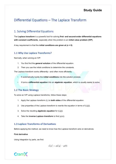 Quick Guides
Differential Equations - The Laplace Transform
Mathematics
27 pagesMar 2026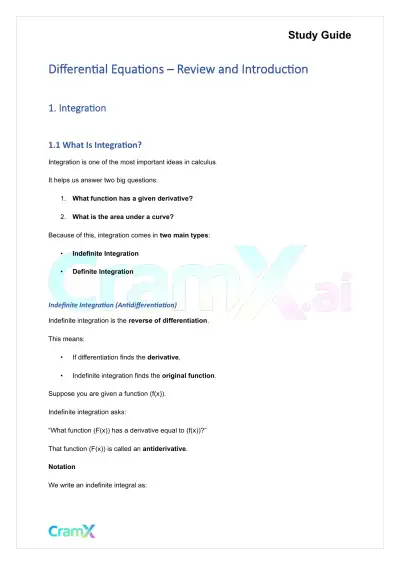 Quick Guides
Differential Equations - Review and Introduction
Mathematics
35 pagesMar 2026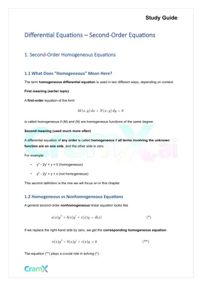 Quick Guides
Differential Equations - Second-Order Equations
Mathematics
45 pagesMar 2026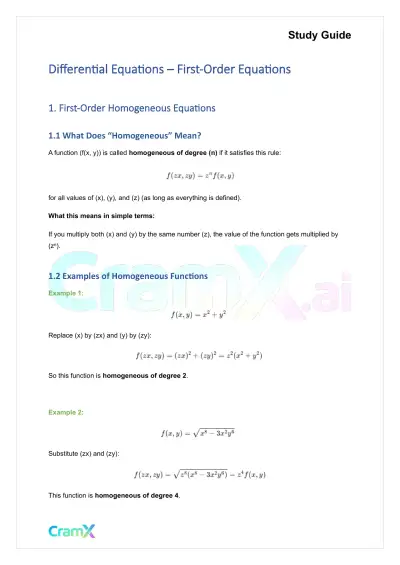 Quick Guides
Differential Equations - First-Order Equations
Mathematics
38 pagesMar 2026 Quick Guides
Differential Equations - Power Series
Mathematics
18 pagesMar 2026 Exam Guides
Test Bank for Precalculus, 6th Edition
Mathematics
1051 pages175downloadsFeb 2025 Textbook Guides
Solution Manual For Introduction To Management Science, 11th Edition
Mathematics
437 pages167downloadsFeb 2025 Textbook Guides
Solution Manual For Derivatives Markets, 3rd Edition
Mathematics
358 pages143downloadsFeb 2025
Study this document with CramX
Once it is in your library, every tool can work from it.