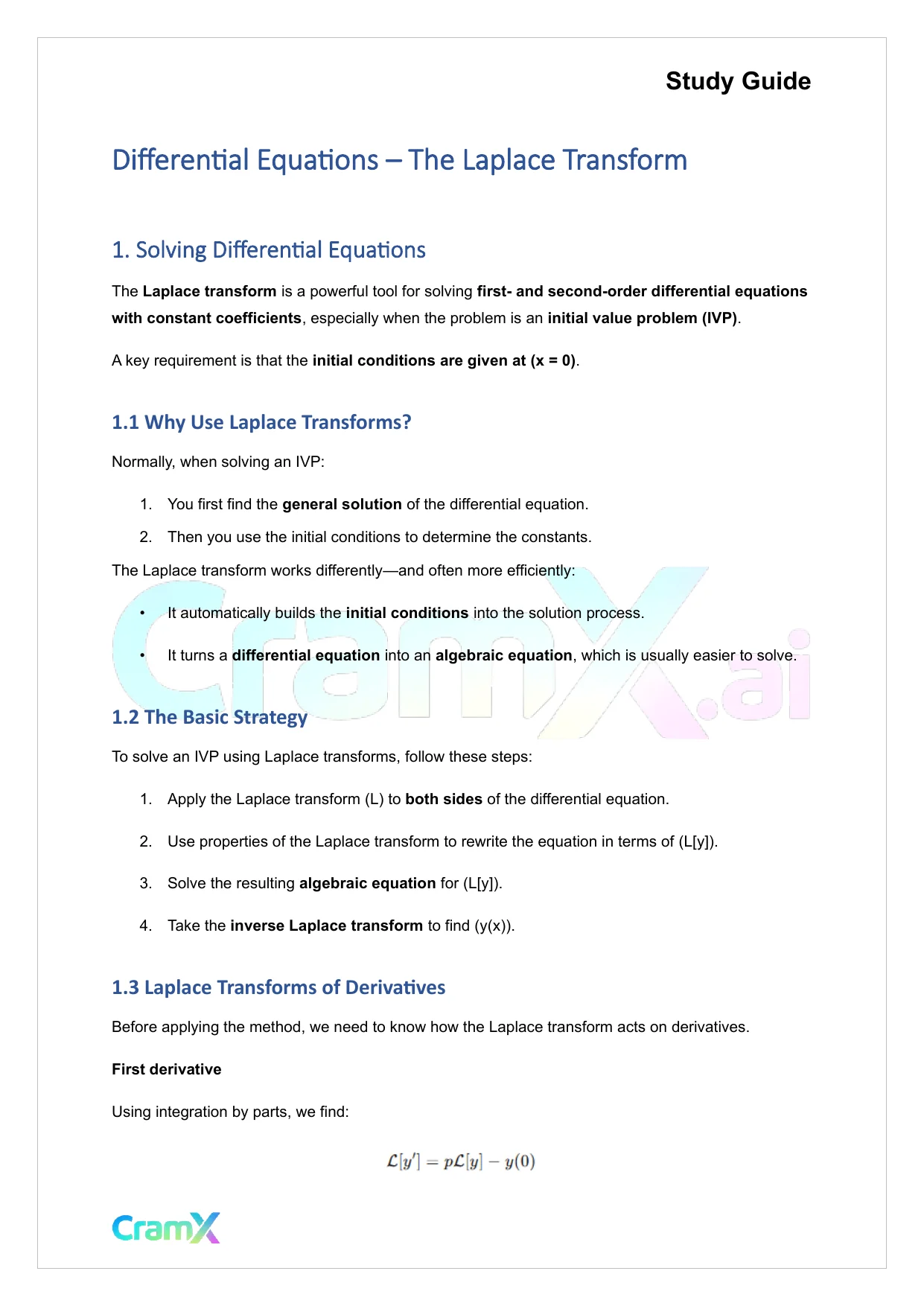
CramX Logo
Differential Equations - The Laplace Transform - Document preview page 1

Differential Equations - The Laplace Transform - Page 1

Document preview content for Differential Equations - The Laplace Transform

Differential Equations - The Laplace Transform

This document provides study materials related to Differential Equations - The Laplace Transform. It may include explanations, summarized notes, examples, or practice questions designed to help students understand key concepts and review important topics covered in their coursework.

Students studying Mathematics or related courses can use this material as a reference when preparing for assignments, exams, or classroom discussions. Resources on CramX may include study notes, exam guides, solutions, lecture summaries, and other academic learning materials.

cenarock
Contributor
0.0
0
about 2 months ago
Preview (9 of 27 Pages)
100%
Log in to unlock
Page 1 of 27
Differential Equations - The Laplace Transform - Page 1 preview imageStudy GuideDifferential EquationsThe Laplace Transform1. Solving Differential EquationsTheLaplace transformis a powerful tool for solvingfirst-and second-order differential equationswith constant coefficients, especially when the problem is aninitial value problem(IVP).A key requirement is that theinitial conditions are given at(x = 0).1.1Why Use Laplace Transforms?Normally, when solving an IVP:1.You first find thegeneral solutionof the differential equation.2.Then you use the initial conditions to determine the constants.The Laplace transform works differentlyand often more efficiently:It automatically builds theinitial conditionsinto the solution process.It turns adifferential equationinto analgebraic equation, which is usually easier to solve.1.2The Basic StrategyTo solve an IVP using Laplace transforms, follow these steps:1.Apply the Laplace transform(L) toboth sidesof the differential equation.2.Use properties of the Laplace transform to rewrite the equation in terms of(L[y]).3.Solve the resultingalgebraic equationfor(L[y]).4.Take theinverse Laplace transformto find(y(x)).1.3Laplace Transforms of DerivativesBefore applying the method, we need to know how the Laplace transform acts on derivatives.First derivativeUsing integration by parts, we find:
Page 2 of 27
Differential Equations - The Laplace Transform - Page 2 preview imageStudy GuideSecond derivativeApplying the same idea again:These formulas are essential because they allow us to replace derivatives with algebraic expressionsinvolving initial values.1.4Common Laplace TransformsMany functions formclosed familiesunder differentiation. This means repeated derivatives staywithin a small group of related functions.Some important examples:Knowing these families makes it easier to recognize inverse transforms later.Example1:First-Order IVPSolve:
Page 3 of 27
Differential Equations - The Laplace Transform - Page 3 preview imageStudy GuideStep 1: Apply the Laplace transformUsing the derivative rule and initial condition:Substitute(y(0) =-5):Step 2: Solve for(L[y])Step 3: Take the inverse Laplace transformUsing partial fractions:Taking inverse transforms:Example2:Second-Order IVPSolve:
Page 4 of 27
Differential Equations - The Laplace Transform - Page 4 preview imageStudy GuideStep 1: Apply the Laplace transformSubstitute initial values:Step 2: SolveAfter partial fraction decomposition and inversion:Example 3:Use Laplace Transforms to Solve the IVPwith initial conditions:We are going to solve this step by step usingLaplace transforms.The big idea is:Take the Laplace transform of both sides.Use the initial conditions.Solve for(L[y]).Take the inverse Laplace transform to find(y(t)).
Page 5 of 27
Differential Equations - The Laplace Transform - Page 5 preview imageStudy GuideStep 1: Take the Laplace TransformApply(L) to both sides:Using linearity:Step 2: Use Laplace FormulasRecall:Now substitute the initial conditions:(y(0) =-1)(y'(0) = 7)So:Step 3: Substitute Everything BackNow simplify:Group like terms:
Page 6 of 27
Differential Equations - The Laplace Transform - Page 6 preview imageStudy GuideStep 4: Solve for(L[y])Step 5: Prepare for Inverse LaplaceRewrite the denominator:Complete the square:So:Rewrite the numerator:So:Rewrite the second fraction to match a standard form:
Page 7 of 27
Differential Equations - The Laplace Transform - Page 7 preview imageStudy GuideStep 6: Take the Inverse Laplace TransformUse standard formulas:Here:(a = 1)(b = 2)So:Final AnswerWhat to NoticeWe used Laplace transforms to turn a differential equation into algebra.Initial conditions were inserted early in the process.Completing the square helped match standard Laplace formulas.The final solution has the form(eat(Acos bt + Bsin bt)), which is typical for complex roots.Example4:Step Functions and Discontinuous InputsThe Laplace transform is especially useful when the forcing function isdiscontinuous, such as astep function.
Page 8 of 27
Differential Equations - The Laplace Transform - Page 8 preview imageStudy GuideFigure 1Figure2Consider:where
Page 9 of 27
Differential Equations - The Laplace Transform - Page 9 preview imageStudy GuideKey Laplace propertyIfthen for any positive constant(k),Applying the methodAfter transforming and solving:Using inverse transforms and the step-function property:This solution matches the expected behavior: nothing happens before(x = 2), and the solutionchanges afterward.SummaryLaplace transforms turn differential equations into algebraic equations.Initial conditions are built directly into the method.The approach works especially well for IVPs with constant coefficients.Step functions and discontinuities are handled naturally using exponential shifts.Inverse transforms rely heavily on recognizing known function families.
Preview Mode

This document has 27 pages. Sign in to access the full document!