

Solution Manual for Business Statistics, 4th Edition
- Statistics
- 582 pages
- Shared February 2025
- 125 downloads
Struggling with problems? Solution Manual for Business Statistics, 4th Edition provides clear, detailed solutions for better learning.
Preview 31 of 582 pages
See the first 31 pages exactly as they appear in the document.
Page 1 Read page 1 as text
I NSTRUCTOR ' S S OLUTIONS M ANUAL FOR B USINESS S TATISTICS L INDA D AWSON University of Washington B USINESS S TATISTICS 4 TH E DITION N OREAN R. S HARPE St. John’s University R ICHARD D. D E V EAUX Williams College P AUL F. V ELLEMAN Cornell University
Page 2 Page 3 Read page 3 as text
Table of Contents Part I Exploring and Collecting Data Chapter 1 Data and Decisions 1 - 1 Chapter 2 Displaying and Describing Categorical Data 2 - 1 Chapter 3 Displaying and Describing Quantitative Data 3 - 1 Chapter 4 Correlation and Linear Regression 4 - 1 Case Study: Paralyzed Veterans of America 4 - 4 9 Part II Modeling with Probability Chapter 5 Randomness and Probability 5 - 1 Chapter 6 Random Variables and Probability Models 6 - 1 Chapter 7 The Normal and Other Continuous Distributions 7 - 1 Part III Gathering Data Chapter 8 Data Sources: Observational Studies and Surveys 8 - 1 Chapter 9 Data Sources:Experiments 9 - 1 Part IV Inference for Decision Making Chapter 10 Sampling Distributions and Confidence Intervals for Proportions 10 - 1 Case Study: Real Estate Simulation Chapter 11 Confidence Intervals for Means 11 - 1 Chapter 12 Testing Hypotheses 12 - 1 Chapter 13 More about Tests and Intervals 13 - 1 Chapter 14 Comparing Two Means 14 - 1 Chapter 15 Inference for Counts: Chi - Square tests 15 - 1 Brief Case : Loyalty Program 1 5 - 27 Part V Models for Decision Making Chapter 16 Inference for Regression 16 - 1 Chapter 17 Understanding Residuals 17 - 1 Chapter 18 Multiple Regression 18 - 1
Page 4 Read page 4 as text
Chapter 19 Buidling Multiple Regression Models 19 - 1 Chapter 20 Time Series Analysis 20 - 1 Case Study : Health Care Costs 20 - 33 Part VI Analytics Chapter 21 Introduction to Big Data and Data Mining 21 - 1 Part VII Online Topics Chapter 22 Quality Control 22 - 1 Chapter 23 Nonparametric Methods 23 - 1 Chapter 24 Decision Making and Risk 24 - 1 Chapter 25 Analysis of Experiments and Observational Studies 25 - 1
Page 5 Read page 5 as text
1-1 Chapter 1 – Data and Decisions SECTION EXERCISES SECTION 1 .1 1. a) Each row represents a different house that was recently sold . It can be described as a case. b) T here are six quantitative variables in each row plus a house identifier for a total of seven variables. 2. a) Each row represents a different transaction (not customer or book). It can be described as a case. b) T here are six quantitative variables plus two identifiers in each row for a total of eight variables . SECTION 1 .2 3. a) House_ID is an identifier (categorical , not ordinal ); Neighborhood is categorical ( nominal); Mail_ZIP is categorical (nominal – ordinal in a sense, but only on a national level); A cres is quantitative (units – acres); Y r _B uilt is quantitative (units – year) ; F ull _M arket _V alue is quantitative (units – dollars); S ize is quantitative (units – sq uare f eet ). b) These data are cross - sectional. Each row corresponds to a house that recently sold so at approximately the same fixed point in time. 4. a) Transaction ID is an identifier (categorical , nominal, not ordinal ); Customer ID is an identifier (cate gorical , nominal ); Date can be treated as quantitative (how many days since the transaction took place, days since Jan. 1 20 09 , for example) or categorical (as month, for example) ; ISBN is an identifier ( categorical , nominal ) ; Price is quantitative (units – dollars); Coupon is categorical ( n ominal); Gift is categorical (nominal); Quantity is quantitative (unit – counts). b) These data are cross - sectional. Each row corresponds to a transaction at a fixed point in time. However , the date of the transaction has been recorded so the data could be reconfigured as a time series. It is likely that the store had more sales in that time period so a time series is not appropriate. SECTION 1 .3 5. It is not specified whether or not the real estate data of Exercise 1 are obtained from a survey . The data would not be from an experiment , a data gathering method with specific requirements . Rather, the real estate major ’s data set was derived from transactional data (on local home sales) . The major concern with drawing conclusions from this data set is that we cannot be sure that the sample is representative of the population of interest ( e.g., all recent local home sales or even all recent national hom e sales ). Therefore, we should be cautious about drawing conclusions from these data about the housing market in general. 6. The student is using a secondary data source (from the Internet). No information is given about how, when, where and why these data were collected or if it was the result of a designed experiment. It is also not stated that the sample is representative of companies . The re are concerns about using these data for generalizing and drawing conclusions because the data could have been collected for a different purpose (not necessarily for developing a stock investment strategy) . Therefore, the student should be cautious about using this type of data to predict performance in the future. CHAPTER EXERCISES 7. The news . Answers will vary. 8. The Internet. Answers will vary. 9. S urvey . The description of the study has to be broken down into its components in order to understand the study. Who – who or what was actually sampled – college students ; What – what is being measured – opinion of electric vehicles: whether there will more electric or gasoline powered vehicles in 2025 and the likelihood of whether they would purchase an electric vehicle in the next 10 years ; Wh en – current ; Where – your location; Why – a utomobile manufacturer wants college student opinions ; How – how was the study
Page 6 Read page 6 as text
1 - 2 Chapter 1 Data and Decisions conducted – survey ; Variables – there are two categorical variable s – what students think about whether or not there will be more electric or gasoline powere d vehicles in 2025 and the second categorical variable is also ordinal – how likely , using a scale, would the student be to buy an electric vehicl e in the next 10 years ; Source – the data are not from a designed survey or experiment ; Type – the data are cross - sectional ; Concerns – none. 10. Your survey . Answers will vary. 11. World databank . Answers will vary but chosen from the following p ossible indicators : • GDP growth (annual %) • GDP (current US$) • GDP per capita (current US$) • GNI per capita, Atlas method (current US$) • Exports of goods and services (% of GDP) • Foreign direct investment, net inflows (BoP, current US$) • GNI per capita, PPP (current international $) • GINI index • Inflation, consumer prices (annual %) • Population, total • Life expectancy at birth, total (years) • Internet users (per 100 people) • Imports of goods and services (% of GDP) • Unemployment, total (% of total labor force) • Agriculture, value added (% of GDP) • CO2 emissions (metric tons per capita) • Literacy rate, adult total (% of people ages 15 and above) • Central government debt, total (% of GDP) • Inflation, GDP deflator (annual %) • Poverty headcount ratio at national poverty line (% of population) 12. Arby’s menu . Who – Arby’s sandwiches; What – type of meat, number of calories (in calories), and serving size (in ounces); Wh en – not specified; Where – Arby’s restaurants; Why – assess the nutritional value of the different sandwiches ; How – information was gathered from each of the sandwiches on the menu at Arby’s, resulting in a census; Variables – there are 3 variables: the number of calories and serving size are quantitative, and the type of meat is categorical; Source – data are not from a designed survey or experiment ; Type – data are cross - sectional; Concerns – none. 13. MBA admissions . Who – MBA applicants (in northeastern U.S. ) ; What – sex, age, whether or not accepted, whether or not they attended, and the reasons for not attending (if they did not accept); Wh en – not specified; Where – a school in the northeastern United States; Why – the researchers wanted to investigate any patterns in female student acceptance and attendance in the MBA program; How – data obtained from the admissions office; Variables – there are 5 variables: sex, whether or not the students accepted, whether or not they attended, and the reasons for not attending if they did not accept (all categorical) and age which is quantitative; Source – data are not from a designed survey or experiment ; Type – data are cross - sectional; Concerns – none. 14. MBA a dmissions II . Who – MBA students (in program outside of Paris ) ; What – each student’s standardized test scores and GPA in the MBA program; Wh en – 200 9 to 20 14 ; Where – outside of Paris ; Why – to investigate the association between standardized test scores and performance in the MBA program over five years (200 9 – 20 14 ); How – not specified; Variables – there are 2 quantitative variables: s tandardized test scores and GPA ; Source – data are not from a designed survey or experiment, data are available from student records ; Type – although the data are collected over 5 years, the purpose is to examine them as cross - sectional rather than as time - series ; Concerns – none.
Page 7 Read page 7 as text
Chapter 1 Data and Decisions 1 - 3 15. Pharmaceutical firm . Who – experimental volunteers ; What – herbal cold remedy or sugar solution, and cold severity; Wh en – not specified; Where – major pharmaceutical firm; Why – scientists were testing the effectiveness of an herbal compound on the severity of the common cold; How – scientists conducted a controlled experiment; Variables – there are 2 variables : t ype of treatment (herbal or sugar solution) is categorical, and severity rating is quantitative; Source – data come f rom a n experiment ; Type – data are cross - sec tional and from a designed experiment ; Concerns – the severity of a cold might be difficult to quantify (beneficial to add actual observations and measurements, such as body temperature). Also, scientists at a pharmaceutical firm could have a predisposed opinion about the herbal solution or may feel pressure to report negative findings about the herbal product. 16. Start - up company. Who – customers of a start - up company; What – customer name, ID number, region of the country (coded as 1 = East, 2 = South, 3 = Midwest, 4 = West ) , date of last purchase , amount of purchase ($), and item purchased; Wh en – present day; Where – not specified ; Why – the company is building a database of customers and sales information; How – assumed that the company records the needed information from each new customer; Variables – there are 6 variables: name, ID number, region of the country, and item purchased which are categorical and date and amount of purchase are quantitative . Date could be coded as categorical as well ; Source – data are not from a designed survey or experiment; Type – data are cross - sectional; Concerns – although region is coded as a number, it is still a categorical variable. 17. Vineyards . Who – vineyards; What – size of vineyard ( most likely in acres), number of years in existence, state, varieties of grapes grown, average case price ($), gross sales ($), and percent profit; Wh en – not specified; Where – not specified ; Why – business analysts hope to provide information that would be helpful to producers of U.S. wines ; How – questionnaire to a sample of growers ; Variables – there are 5 quantitative variables: the size of vineyard (acres), number of years in existence, average case price ($), gross sales ($) ; there are 2 categorical variables: s tate and variety of grapes grown; Source – data come from a designed survey; Type – data are cross - sectional; Concerns – none. 18. Spectrem group polls . Who – not completely clear. Probably a sample of affluent and retired people ; What – p et preference, number of pets, services and product s bought for pets (from a list) ; Wh en – not specified; Where – United States; Why – provide s ervice s for the affluent ; How – survey; Variables – there are 3 categorical variables: p et preference, list of pets and list of services and products bought for pet ; Source – data from a designed survey; Type – data are cross - sectional; Concerns – none. 19. EPA . Who – every model of automobile in the United States; What – vehicle manufacturer, vehicle type (car, SUV, etc.), weight (probably pounds), horsepower (units of horsepower), and gas mileage (miles per gallon) for city and highway driving; Wh en – the information is currently collected; Where – United States; Why – the EPA uses the information to track fuel economy of vehicles; How – a mong the data EPA analysts collect from the automobile manufacturers are the name of th e manufacturer (Ford, Toyota, etc .), vehicle type….” ; Variables – there are 6 variables : v ehicle manufacturer an d vehicle type are categorical variables ; w eight, horsepower , and gas mileage for both city and highway driving are quantitative variables; Source – data are not from a designed survey or experiment ; Type – data are cross - sectional; Concerns – none. 20. Consumer Reports . Who – 46 models of smart phones ; What – brand, price (probably dollars), display size (probably inches) operating system, camera image size (megapixels) , and memory card slot (yes/no) ; When – not specified ; Where – not specified ; Why – the information was compiled to provide information to readers of Consumer Reports; How – not specified; Variables –– there are a total of 6 variables: price, display size and image size are quantitative variables; brand and operating system are categorical variables , and memory card slot is a nominal variable ; Source – not specified ; Type – the data are cross - sectional; Concerns – this many or may not be a representative sample of smart phones , or includes all of them, we don’t know. This is a rapidly changing market, so their data are at best a snapshot of the state of the market at this time. 21. Zagat . Who – restaurants ; What – % of customers liking restaurant, average meal cost ($), food rating (0 - 30), decor rating (0 - 30), service rating (0 - 30) ; Wh en – current ; Where – not specified ; Why – service to provide information for consumers ; How – not specified; Variables – there are 5 variables: % liking and average cost
Page 8 Read page 8 as text
1 - 4 Chapter 1 Data and Decisions are quantitative variables; r atings (food, decor and service) are ordered categories , therefore, ordinal variables ; Source – not specified ; Type – the data are cross - sectional . 22. L.L. Bean . Who – catalog mailings ; What – number of catalogs mailed out, square inches in catalog, and sales ($ million) in 4 weeks following mailing; Wh en – current; Where – L.L. Bean ( United States ) ; Why – to investigate association among catalog characteristics, timing, and sales; How – collect ion of internal data; Variables – there are 3 variables : n umber of catalogs, square inches in catalog, and sales are all quantitative variables ; Source – not specified ; Type – data are cross - sectional; Concerns – none. 23. Stock market . Who – students in an MBA statistics class; What – total personal investment in stock market ($), number of different stocks held, total invested in mutual funds ($), and the name of each mutual fund; Wh en – not specified; Where – a business school in the northeast US; Why – the information was collected for use in classroom illustrations; How – an online survey was conducted, participation was probably required for all members of the class; Variables – there are 4 variables : t otal persona l investment in stock market , number of different stocks held, tot al invested in mutual funds are quantitative variables ; t he name of each mutual fund is a categorical variable; Source – data come from a designed survey; Type – data are cross - sectional . 24. Theme park sites . Who – potential theme park locations in Europe ; What – country of site, estimated cost ( probably € ), potential population size (counts), size of site ( probably hectares), whether or not mass transportation within 5 minutes of site; Wh en – 20 13 ; Where – Europe; Why – to present to potential developers on the feasibility of various sites; How – not specified; Variables – there are 5 variables : c ountry of site and whether or not mass transportation is within 5 minutes of site are both categorical variables ; e stimated cost , potential population size and size of site are quantitative variables ; Source – data are not from a designed survey or experiment; Type – data are cross - sectional . 25. Taxi data . Who – taxi rides in NYC ; What – vendor ID , pickup time , dropoff time , number passengers, trip distance, pickup longitude and latitude, dropoff longitude and latitude, fare amount, tip amount, toll amount, total amount ; Where – New York City ; Why – market analysis of taxi rides ; How – the New York City Taxi and Limousine Commission records the trip information ; Variables –– there are 13 variables : number of passengers, trip distance, pickup and dropoff longitude and latitude, fare amount, tip amount, toll amount, total amount, and the date and time of pickup are quantitative (dates c ould also be considered categorical) ; Sou rce – NYC Taxi and Limousine Commission ; Type – data are cross - sectional ; Concerns – none. 26. Dalia Research . Who – 43,034 people worldwide who responded to the Dalia survey ; What – ID #, age, plan to purchase car, city/rural, mobile device, education, gender, latitude, longitude, country, town size, household size ; Wh en – not specified in problem ; Where – worldwide ; Why – Dalia collects data about a wide variety of topics for market research purposes ; How – survey sent to an unspecified number of people worldwide ; Variables – there are 12 variables in the subset of data presented : age, latitude and longitude are quantitative. Plan to purchase car, city or rural, mobile device, education, gender, country, and town size are cate gorical. ID is an identifier. Town size, household size, and education are also ordinal ; Source – survey results ; Type – data are cross - sectional ; Concerns – none. 27. Mortgages . Each row represents each individual mortgage loan. Headings of the columns would be: loan number (the row identifier), last 4 numbers of the borrower’s social security number, mortgage amount , borrower’s name. 28. Employee performance . Each row represents each individual employee. Headings of the columns would be: Employee ID Number (to identify the row instead of name), contract average ($), supervisor’s rating (1 - 10), and years with the company. 29. Company performance . Each row represents a week. Headings of the columns would be: week number of the year (to identify each row), sales prediction ($), sales ($), and difference between predicted sales and realized sales ($).
Page 9 Read page 9 as text
Chapter 1 Data and Decisions 1 - 5 30. Command performance . Each row represents a Broadway show. Headings of the columns would be: the show name (identifies the row), profit or loss ($), number of investors and investment total ($). 31. Car sales . Cross - sectional are data taken from situations that vary over time but measured at a single time instant . This problem focuses on data for September only which is a single time period. Therefore, the data are cross - sectional. 32. Motorcycle sales. Time - series data are measured over time. Usually the time intervals are equally - spaced (e.g. every week, every quarter, or every year). This problem focuses on the number of motorcycles sold by the dealership in each month of 20 14 ; therefore, the data are measure d over a period of time and are time series data. 33. Forestry . Time - series data are measured over time. Usually the time intervals are equally - spaced (e.g. every week, every quarter, or every year). This problem focuses on the average diameter of trees brought to a sawmill in each week of a year; therefore, the data are measure d over a period of time and are time - series data. 34. Baseball . Cross - sectional are data taken from situations that vary over time but measured at a single time instant . This problem focuses on data for attendance of the third World Series game. Therefore, the data are cross - sectional.
Page 10 Read page 10 as text
1 - 6 Chapter 1 Data and Decisions Ethics in Action Sarah’s dilemma: The company RSPT Inc. is having Sarah compare their strategies to other companies. However, they could influence the outcome by funding the research and providing free software. In addition, Sarah may feel obliged to favor RSPT Inc. because they were generous in providing her r esearch tools and funding. The company may put pressure on her to favor their methods over others because of their close relationship. The undesirable consequences are that the results are not completely objective and bias exists due to the funding circums tances. One possible solution would be to find other grants outside of RSPT Inc. but not connected to any of the companies being compared. This might also be true of the software. It is important in a scientific study to be completely objective and not be influenced by one of the clients being examined. Jim’s dilemma: Statistics and data can often be manipulated to produce a desired result that can “fudge” result s and present a more desirable outcome. The scientific method is constructed to be objective if the rules are followed. The objective of Jim’s study was to increase the percentage of clients who viewed their advisory services as outstanding, not increase th e overall satisfaction average. In presenting an increased average , Jim is not being honest about the specific results of his study with respec t to his objective. He should be honest about the decrease in the “outstanding” category. One possible solution might be to compare the number of responses in each survey to see if there is a discrepancy that could explain the change. In addition, he could point out the large increase in the “above average” category (10% to 40%) which shows a h uge improvement. Many people may be unwilling to give the highest rating on an intermediate basis but would be willing to identify an improvement. For further information on the official American Statistical Association’s Ethical Guidelines, visit: http://www.amstat.org/about/ethicalguidelines.cfm The Ethical Guidelines address important ethical considerations regarding professionalism and responsibilities. Brief Case – Credit Card Bank List the W’s for these data : Who – bank cardholders What – monthly credit card charges made by cardholder from August 20 16 through April 2017, marketing segment, industry segment, amount of spend lift after promotion, average spending on card pre - and post - promotion, whether or not cardholder is a retail or travel customer , and the type of spending habits. Why – to determine customer spending habits and what types of offers are being taken advantage of and in what way. When – most likely in 20 17 Where – although not specified, most likely national data collected in U.S. How – demographic data most likely collected when credit card account was opened and spending data collected during transactions Classify each variable as categorical or quantitative; if quantitative identify the units: Offer Type – categorical Enrollment Required – categorical Charges August 20 16 – quantitative ($) Charges September 20 16 – quantitative ($) Charges October 20 16 – quantitative ($) Charges November 20 16 – quantitative ($) Charges December 20 16 – quantitative ($) Charges January 20 17 – quantitative ($) Charges February 20 17 – quantitative ($)
Page 11 Read page 11 as text
Chapter 1 Data and Decisions 1 - 7 Charges March 20 17 – quantitative ($) Charges April 20 17 – quantitative ($) Opportunity Segment – categorical Industry Segment – categorical Combined Segment – categorical Spend Lift – quantitative ($)
Page 12 Read page 12 as text
2-1 Chapter 2 – D isplaying and Describing Categorical Data SECTION EXERCISES SECTION 2 .1 1. a) Frequency table: b) Relative frequency table (divide each number by 512 and multiply by 100): 2. a) Frequency table: b) Relative frequency table: SECTION 2 .2 3. a) b) None AA BA MA PhD 164 42 225 52 29 None AA BA MA PhD 32.03% 8.20% 43.95% 10.16% 5.66% Under 6 6 to 9 10 to 14 15 to 21 Over 21 45 83 154 18 170 Under 6 6 to 9 10 to 14 15 to 21 Over 21 9.57% 17.66% 32.77% 3.83% 36.17%
Page 13 Read page 13 as text
2 - 2 Chapter 2 Visualizing and Describing Categorical D ata c) 4. a) b) c)
Page 14 Read page 14 as text
Chapter 2 Visualizing and Describing Categorical D ata 2 - 3 5. a) Most employees have either a bachelor’s degree (44%) or no college degree (32%). About 10% have master’s degrees, 8% have associate’s degrees, and nearly 6% have PhDs. b) It is difficult to generalize these results to any other division of the company or to any other company. These data were collected from only one division. Other divisions and companies might have vastly different educational requirements for their employees and therefore distributions of educational levels. 6. a) Approximately 1 3 of the viewers were 10 – 14 years old. Over a third (36%) of the viewers were over the age of 21, many of whom could be parents accompanying their children. Slightly over 50% of the viewers were children and younger teenagers from 6 to 14 years of age. About 10% of the viewers were younger children under 6 years of age. Only 4% were older teenagers to young adults from 15 to 21 years of age. b) We do not know whether these audiences are representative. No information is given about how the locations were selected, what time of day the interviews were conducted , etc. Moreover, we don’t know how many individuals did not agree to be interview ed . Are teenagers and young adults from 15 to 21 years of age underrepresented in the sample because the film was not appealing to this age group or because they declined to be interviewed ? SECTION 2 .3 7. a) b) Yes. 8. a) b) Yes. Totals < 1 year 95 1 - 5 years 205 more than 5 years 212 None AA BA MA PhD 164 42 225 52 29 Totals Never 350 Once 78 More than Once 42 Under 6 6 to 9 10 to 14 15 to 21 Over 21 45 83 154 18 170
Page 15 Read page 15 as text
2 - 4 Chapter 2 Visualizing and Describing Categorical D ata SECTION 2.4 9. a) b) N o. The distributions look quite different. More than 2/3 of those with no college degree have been with the company longer than 5 years, but almost none of the PhDs (less than 7%) have been there that long. It appears that within the last few years the company has hired b etter educated employees. c) d) It is easier to see the differences in the distributions in the stacked bar chart . e) A mosaic plot would display the different counts for each degree type. Areas of the plot representing each cell would then reflect the cell counts accurately. 10. a) b) The vast majority of viewers hadn’t seen the movie before except for the 10 - to 14 - year - old group, where nearly half (45.5%) had seen the movie at least once. (%) None AA BA MA PhD < 1 year 6.1 7.1 22.2 38.5 41.4 1 - 5 years 25.6 21.4 49.8 51.9 51.7 more than 5 years 68.3 71.4 28.0 9.6 6.9 (%) Under 6 6 to 9 10 to 14 15 to 21 Over 21 Never 86.7 72.3 54.5 88.9 88.8 Once 6.7 24.1 24.7 11.1 8.8 More than once 6.7 3.6 20.8 0 2.4
Page 16 Read page 16 as text
Chapter 2 Visualizing and Describing Categorical D ata 2 - 5 c) d) It is easier to see the differences in the distribution in the stacked bar chart. The stacked bar chart makes the 10 to 14 year old age group (and to a less er extent the 6 to 9 year old age group) stand out as having a larger percentage of viewers who have seen the movie at least once before compared to the other age groups. e) A mosaic plot would display the different counts in each age group accurately as well, providing a better representation of the counts in the table. CHAPTER EXERCISES 11. Graphs in the news . Answers will vary. 12. Graphs in the news, part 2 . Answers will vary. 13. Tables in the news . Answers will vary. 14. Tables in the news, part 2 . Answers will vary. 15. U.S. market share. a) Yes, this is an appropriate display for these data because all categories of one variable (sellers of carbonated drinks) are displayed. The categories divide the whole and the category Other combines the smaller shares. b) The company with the largest share is Coca - Cola. 16. Brand value . a) Yes, this is an appropriate display for these data. The variable which is categorical (distributors of carbonated beverages ) are displayed and dollar value easily readable . b) The company with the smallest share is Dr. Pepper . c) Red Bull slightly edges out Pepsi.
Page 17 Read page 17 as text
2 - 6 Chapter 2 Visualizing and Describing Categorical D ata 17. Market share again. a) The pie chart does a better job of comparing portions of the whole. b) The “Other” category is missing and without it, the results could be misleading. 18. Brand value again. a) T he bar chart does a better job . T he close categories are hard to compare directly in a pie chart because they are almost the same size pie segments . b) Too close to tell from the pie chart. Much easier to see from the bar chart . 19. Insurance company. a) Yes, it is reasonable to conclude that deaths due to heart OR respiratory diseases is equal to 30.3% plus 7.9%, which equals 38.2%. The percentages can be added because the categories do not overlap. There can only be one primary cause of death. b) The percentages listed in the table only add up to 73.7%. Therefore, other causes must account for 26.3% of U.S. deaths. c) An appropriate display could either be a bar graph or a pie graph, using an “Other” category for the remaining 26.3% causes of death. 20. Financial satisfaction a) Answers may vary . Side - by - side bar charts , stacked bar charts , or mosaic plots would all be good visualizations. A comparison of percentages by level of satisfaction is shown in the following segmented bar chart. It is appropriate to compare percentages rather than individual numbers. Based on the given data, the comparison between females and males show that both genders have very comparable percentages for levels of satisfaction. It would not be reasonable to conclude that females are less satisfied than males with their financial situation . b) It would not be reasonable to conclude that there are more than 50% males in the United States from the data provided because the data represent a sample, not the whole.
Page 18 Read page 18 as text
Chapter 2 Visualizing and Describing Categorical D ata 2 - 7 21. B2B . Cisco and Polycom are close to each other, battling for first place in the Netherlands, and the remainder of the market is fragmented. A pie chart or bar chart would be appropriate. 0.31 0.30 0.38 0.36 0.16 0.17 0.13 0.14 0.03 0.02 M A L E F E M A L E Very satisfied Somewhat satisfied Somewhat dissatisfied Very dissatisfied No Answer Polycom 31% Cisco 33% Lifesize 11% Siemens Others 22%
Page 19 Read page 19 as text
2 - 8 Chapter 2 Visualizing and Describing Categorical D ata 22. Toy makers . a) Answers may vary. Sales of toys grew nearly 15.9% from 2013 to 2016. T he only categor y that did not show growth was Arts & Crafts . Outdoor & Sports Toys and Infant/Toddler/Preschool Toys were the largest two categories across the years , followed by Dolls closely behind in third place. In terms of percentages, between 2013 and 2016, Outdoor & Sports Toys ( 23% increase), Games/Puzzles ( 43 % increase), and Dolls ( 25 % increase) grew the most. b) Answers may vary. Plotted as raw values ($) or as a stacked bar graph, it is difficult to see the differences. Computing the percent of total by year and using that value in a bar graph comparing percent by years, reveals changes from 2013 to 2016 for each category. Specifically, Outdoor & Sports Toys , Infant/Toddler/Preschool Toys, and Dolls have the highest percentages for 2016. 23. Job satisfaction . a) The percentages don’t total 100%. Others either refused to answer or didn’t know. b) Bar chart: 0% 2% 4% 6% 8% 10% 12% 14% 16% 18% 20% Percent of Toy Sales 2013 (%) 2016 (%)
Page 20 Read page 20 as text
Chapter 2 Visualizing and Describing Categorical D ata 2 - 9 c) A pie chart would not be appropriate with the data as is because the percentages do not represent parts o f a whole and do not total 100% . A pie chart would work if “Other” category is added. 24. Small business hiring . a) The percentages total 98 %. The other 2% either didn’t answer or didn’t know. b) Bar chart: c) A pie chart would not be appropriate because the percentages do not represent parts of a whole and do not total 100%. An “Other” category would have to be added. d) (Answer s will vary) Half (50%) of the respondents said that their cash flow was very or somewhat good (37% said somewhat). Only 27% said somewhat or very poor. 25. Environmental hazard 201 6 . The bar chart shows that G rounding and Collisions are the most frequent cause s of oil spillage for these 4 60 spills and allows the reader to rank the other types as well. If being able to differentiate between close counts is required, use the bar chart. The pie chart is also acceptable as a display and makes it easier to see that Grounding and Collisions make up around 60% of the total causes of spillage but it is 0% 10% 20% 30% 40% 50% Very satisfied Somewhat satisfied Somewhat dissatisfied Very dissatisfied Other
Page 21 Read page 21 as text
2 - 10 Chapter 2 Visualizing and Describing Categorical D ata harder to determine the causes that are close to each other, such as Grounding and Collisions or Hull Failure vs. Fire/ Explosion . To showcase the causes of oil spills as a fraction of all 4 60 spills, use the pie chart. 26. Olympic medals . a) If we treat the number of medals as the category, there are too many categories -- most of them empty. b) One alternative is to show only the bars for medal counts that have occurred. The risk here is that a reader might not notice the missing counts. 0 10 20 30 40 50 60 70 80 0 10 20 30 40 60 80 90 250 # OF COUNTRIES MEDALS/CAPITA > 0
Page 22 Read page 22 as text
Chapter 2 Visualizing and Describing Categorical D ata 2 - 11 27. Importance of wealth . a) India 76.1% - USA 45.3% = 30.8% , almost 31% b) The vertical axis on the display starts at 40% which makes the comparison between countries difficult and the areas disproportionate. For example, the India bar looks about 5 - 6 times as big as the USA bar when in fact the actual values are not even twice as big. c) The display would be improved by starting the vertical axis at 0%, not 40%. d) e) The percentage of people who say that wealth is important to them is highest in China and India (over 70%), followed by France (close to 60%) and then the USA and U.K. where the percentages were close to 45%. 28. Importance of power . a) The percentages don’t add up to 100% so a pie chart is not appropriate. Showing the pie chart three dimensionally on a slant violates the a rea p rinciple and makes it much more difficult to compare fractions of the whole. b) A bar chart is more appropriate. 40.00% 45.00% 50.00% 55.00% 60.00% 65.00% 70.00% 75.00% 80.00% China France India U.K. U.S.
Page 23 Read page 23 as text
2 - 12 Chapter 2 Visualizing and Describing Categorical D ata c) The percentage of people who say that power is important to them is highest in India (over 75%), followed by China (close to 72%) and then France (almost 60%). The lowest percentages occur in USA and the UK (both close to 45%). 29. G E financials . a) These are column percentages because the column sums add up to 100% and the row percentages add up to more than 100%. b) A stacked bar chart is appropriate. c) Over 50% of GE’s revenue comes Power, Aviation, and Healthcare , except in 2012, which had a major drop in Aviation revenue and a major increase in Other. In a typical year, 45% of revenue is accounted by Other sources. 30. Real estate pricing . a) These are column percentages because the column sums add up to 100% and the row percentages add up to more than 100%. b) 2.4% c) This cannot be determined. We are only given the percentages of size within each Price category. d) Small 61.5% + Med Small 30.4% = 91.9%. e) Larger houses appear to cost more . A stacked bar chart is shown below illustrating the changing conditional distributions. 0% 10% 20% 30% 40% 50% 60% 70% 80% 90% 100% 2015 2014 2013 2012 2011 Power Aviation Healthcare Other
Page 24 Read page 24 as text
Chapter 2 Visualizing and Describing Categorical D ata 2 - 13 31. Stock performance . a) 4 5.1 % ( 164 +48) / 470 ) b) 34.9 % (1 64) /4 70 ) c) 5.3 % ( 25 /4 7 0) d) 59.8 % ( 48 +2 33 ) / 470 ) e) 4 1.3 % (1 64 / 397 ) f) 65.8% 48 / (48+25 ) g) Companies that reported a positive change on a single day were more likely to report a negative change for the year than companies who reported a negative change on a single day . 32. New product . a) 4.0% (56/1415) b) 34% (481/1415) c) 3.7% (18/481) d) 32.1% (18/56) e) Marginal Distributions – total % of the categories: Students 64 .0 %; Faculty/Staff 23.9%; Alumni 4 .0 %; Town Residents 8.2%. f) Conditional Distributions – percentages for Very Likely column: Students 66.5%; Faculty/Staff 20.4%; Alumni 3.7%; Town Residents 9.4%. g) The likelihood to buy seems independent of campus group (compare percentages for Very Likely in each category). However, there are more students, so focusing advertising in that group may have a greater impact on revenue. 33. Foreclosures 2016 . a) 1 0 . 1 % ( 203,108 / 2,020,354 ) b) 33 . 4 % ( 2,300,000 / 6,891,060 ) c) 1 2 . 5 % ( 575,378 / 4,599,817 ) d) Overall, the change was – 71.0%. On a compound annual growth rate basis, this is – 26.6% per year. e) Answers may vary. Two things stand out: the numbers seem rounded for 2012 and not for the other years. Two numbers in 2014 and 2015 are identical.
Page 25 Read page 25 as text
2 - 14 Chapter 2 Visualizing and Describing Categorical D ata 34. Appl financials . a) R&D % 2014 : 4.2 % ( 6,041,000 / 144,265,000 ) ; 2016: 5.9 % ( 10,045,000 / 171,300,000 ) b) Tax % 2015: 1 0.5 % ( 1 9 , 121 ,000 /1 8 1, 606 ,000 ) ; 2016: 9 . 2 % ( 15,685,000 / 171,300,000 ) c) In absolute dollars, SG&A has increased, but because total expenses have increased, as a percentage of total expenses, SG&A has fallen slightly. d) e) 35. Movie ratings . a) Conditional distribution (in percentages) of movie ratings for action films: R or NC - 17 PG - 13 PG G Total Action 44.1% 52.9% 2.9% 0.0% 100.0% b) Conditional distribution (in percentages) of movie ratings for PG - 13 films: 2014 2015 2016 Cost of Revenue 77.8% 77.1% 76.7% Research & Development 4.2% 4.4% 5.9% Selling, General, & Administrative 8.3% 7.9% 8.3% Income Tax Expense 9.7% 10.5% 9.2% PG - 13 Action 15.1% Comedy 21.8% Drama 51.3% Thriller/Suspense 11.8% 0% 10% 20% 30% 40% 50% 60% 70% 80% 90% 100% Cost of Revenue Research & Development Selling, General, & Administrative Income Tax Expense 2014 2015 2016
Page 26 Read page 26 as text
Chapter 2 Visualizing and Describing Categorical D ata 2 - 15 c) Depending on what you want to emphasize, either segmented bar chart shown below is appropriate. Placing Genre on the x - axi s emphasizes that Dramas are the most commonly made film type. Placing MPAA Rating on the x - axis show that R (or NC - 17) movies are the most commonly made. 0 20 40 60 80 100 120 140 160 180 Action Comedy Drama Thriller/Suspense R or NC-17 PG-13 PG G 0 50 100 150 200 250 R or NC-17 PG-13 PG G Action Comedy Drama Thriller/Suspense
Page 27 Read page 27 as text
2 - 16 Chapter 2 Visualizing and Describing Categorical D ata d) Genre and Rating do not appear to be independent. It appears that it is more likely for a Drama or a Comedy to be rated PG than Action or Thriller. Similarly, Thriller/Suspense movies are more likely to be rate R. 36. CyberShopping . a) Conditional distribution (in percentages) of income distribution for those who do NOT compare prices on the Internet : b) Conditional distribution (in percentages) of income distribution for those who DO compare prices on the Internet : Under $30K 31.4 % (207/660) $30K - $50K 17.4 % (115/660) $50K - $75K 20.3 % (134/660) Over $75K 30.9 % (204/660) c) Bar chart: d) A nswers may vary. Comparison shopping is more common among those with higher incomes. 37. MBAs . a) 62.7% (168/268) b) 62.8% (103/164) c) 62.5% (65/104) d) The marginal distribution of origin: 23.9% from Asia; 1.9% from Europe; 7.8% from Latin America; 3.7% from the Middle East; 62.7% from North America. Under $30K 36.6 % ( 625 / 1708 ) $30K - $50K 23 .8% (406/1708) $50K - $75K 15.2 % (260/1708) Over $75K 24.4 % (417/1708)
Page 28 Read page 28 as text
Chapter 2 Visualizing and Describing Categorical D ata 2 - 17 e) The column percentages: Two - Yr Evening Total Asia/Pacific Rim 18.90 31.73 23.88 Europe 3.05 0.00 1.87 Latin America 12.20 0.96 7.84 Middle East/Africa 3.05 4.81 3.73 North America 62.80 62.50 62.69 Total 100.00 100.00 100.00 f) They are not independent. For example, there is less than a 19% chance (31/164) that a randomly selected Two - Year MBA student is an Asian/Pacific Rim student. However, there is more than a 31% chance (33/104) that a randomly selected Evening MBA student is an Asian/Pacific Rim stud ent. This is over a 50% increase in the likelihood that a student is an Asian/Pacific Rim student. In addition, the percentage from Latin America in Two - Year programs is 12.2% while for thos in the Evening programs is leass than 1%. Thus knowing the kind o f MBA program does affect the likelihood of the origin of the MBA student. 38. MBAs, part 2 . a) 32.1% (86/268) b) 29.3% (48/164) c) 36.5% (38/104) d) There seems to be a slightly higher percentage of Evening MBAs who are women. This may be because women have other commitments during the day (such as work, family, etc.) that limit their choices. 39. Top producing movies . a) 2 . 0 % ( 135 / 6897 ) b) 2 . 5 % (1 8 / 716 ) c) 2 . 0 % (140/6897) d) 20.0 % ( 943 / 4,718 ) e) 54.5 . 0 % ( (592+879+3) / 2,703) f) More movies were unrated in the 2011 - 201 5 time period than the 2006 - 2010 period. However, of the movies that were rated, the distributions are similar. There are slightly more R rated movies in the 2006 - 2010 time period but this could be because makers of R rated movies chose instead to release t hem unrated in the later time period (2011 - 201 5 ). 40. Movie admissions 201 6 . a) 3 3 . 4 % ( (16.2+19.9) / 10 8.1 ) b) 56 . 7 % ( (5.4+7.2+8) / 3 6.3 ) c) 6. 5 % ( 7 /1 0 8.1 ) d) 1 4 . 9 % ( 5.1 / 3 4.3 ) e) 4. 7 % ( 5.1 / 10 8.1 ) f) The conditional age distribution - each value is divided by the total for that year: NC - 17 R PG - 13 PG G Not Rated 2006 - 2010 0.15% 33.11% 20.80% 9.87% 2.13% 33.94% 2011 - 201 5 0.16% 30.36% 19.64% 8.40% 1.81% 39.63%
Page 29 Read page 29 as text
2 - 18 Chapter 2 Visualizing and Describing Categorical D ata 2 - 11 12 - 17 18 - 24 25 - 39 40 - 49 50 - 59 60+ 2016 8.5% 14.9% 19.8% 22.0% 9.1% 11.6% 14.0% 2015 8.5% 15.5% 16.6% 21.6% 13.1% 9.9% 14.9% 2014 7.2% 14.7% 18.7% 18.9% 15.2% 11.2% 14.1% The age distribution stayed fairly constant between the three years. The largest percentage of movie goers are in the age groups 18 - 24 and 25 - 39 consistently. There seems to be a substantial decline in the 40 - 49 age group and older. Other changes seem to more like random fluctuations and not extreme. 41. Tattoos . The study by the University of Texas Southwestern Medical Center provides evidence of an association between having a tattoo and contracting hepatitis C. Approximately 33% of the subjects who were tattooed in a commercial parlor had hepatitis C, compared with 13% of those tattooed elsewhere, and only 3.5% of those with no tattoo. If having a tattoo and having hepatitis C were independent, we would have expected these percentages to be roughly the same. 42. Poverty and region 201 5 . The percentage of people living below poverty level in the four regions are : 12. 4 , 1 1 .7, 1 5 . 3 and 1 3 . 3 , respectively. Although the rates are similar, there do seem to be higher rates in the South and West than in the Northeast and Midwest. 43. Being successful . a) 51.4 % ( (139+273)/802) b) Men are slightly higher . Young men: 5 4.3 % ( (163+346)/937) c) The distributions are similar, but slightly more men say that a high - paying job is “very” important, and slightly more women say that a high - paying job is “somewhat” important . 44. Minimum wage workers . a) 20.3 % (Count for 16 - 24 divided by Total Female : 7701/37,972 ) b) It can be seen from the side - by - side bar graph below that t he proportion of female workers who work at minimum wage or less is nearly twice that of men at every age group. 0% 10% 20% 30% 40% 50% 60% 70% 80% 90% 100% Tattoo Done in Commercial Parlor Tattoo Done Elsewhere No Tattoo Has Hepatitis C No Hepatitis C
Page 30 Read page 30 as text
Chapter 2 Visualizing and Describing Categorical D ata 2 - 19 45. Moviegoers and ethnicity . a) Caucasian Hispanic African - American Other Population 66.0% (204.6/310) 16.0% (49.6/310) 12.0% (37.2/310) 6.0% (18.6/310) Moviegoers 63.0% (88.8/141) 19.0% (26.8/141) 12.0% (16.9/141) 6.0% (8.5/141) Tickets 56.0% (728/1300) 26.0% (338/1300) 11.0% (143/1300) 7.0% (91/1300) b) The distributions of moviegoers are quite similar to the population as a whole, but Hispanics appear to buy proportionally more tickets and Caucasians fewer. Hispanics appear to go to the movies more often, on average, than Caucasians . 46. Department store . a) Low 20.0%; Moderate 48.9%; High 31.0%. b) Under 30: Low 27.6%; Moderate 49.0%; High 23.5% 30 - 49: Low 20.7%; Moderate 50.8%; High 28.5% Over 50: Low 15.7%; Moderate 47.2%; High 37.1% - 0.02 0.04 0.06 0.08 0.10 0.12 16-24 25-34 35-44 45-54 55-64 65+ Men Women
Page 31 Read page 31 as text
2 - 20 Chapter 2 Visualizing and Describing Categorical D ata c) d) As age increases, the percentage of customers reporting a high frequency of shopping increases, and the percentage who report a low frequency of shopping decreases. e) No. An association between two variables does not imply a cause - and - effect relationship. 47. Success II . Needs changes a) 53.0% b) Number of 18 - 34 yr olds who think being successful is one of the most important things = 44.7% 48. Income and pets . a) No, the income distributions of households by pet ownership wouldn’t be expected to be the same. Caring for a horse is much more expensive, generally, than caring for a dog, cat, or bird. Households with horses as pets would be expected to be more common in the higher in come categories. b) Column percentages (add up to 100%). c) No. Among horse owners, there are relatively fewer households in the lowest income bracket and relatively more households in the highest income bracket. In the middle income ranges, the percentages are about the same for each of the different types of pets . 49. Insurance company, part 2 . a) The marginal totals were added. 160 of 1300 or 12.3% had a delayed discharge. b) Major surgery patients were delayed 15.3% of the time. Minor surgery patients were delayed 6.7% of the time. c) Large Hospital had a delay rate of 13%. Small Hospital had a delay rate of 10%. The small hospital has the lower overall rate of delayed discharge. d) Large Hospital: Major Surgery 15% and Minor Surgery 5%. Small Hospital: Major Surgery 20% and Minor Surgery 8%. e) Yes, while the overall rate of delayed discharge is lower for the small hospital, the large hospital did better with both major and minor surgery. f) The small hospital performs a higher percentage of minor surgeries than major surgeries. 250 of 300 surgeries at the small hospital were minor (83%). Only 200 of the large hospital’s 1000 surgeries were minor (20%). Minor surgery had a lower delay rate than major surgery (6.7% to 15.3%), so the small hospital’s overall rate was artificially inflated. The larger hospital is the better hospital whe n comparing discharge delay rates. Large Hospital Small Hospital Total Major surgery 120 of 800 10 of 50 130 of 850 Minor surgery 10 of 200 20 of 250 30 of 450 Total 130 of 1000 30 of 300 160 of 1300
551 more pages in the full document
Unlock it once and it stays in your library, ready to chat with or turn into flashcards.
Unlock the full documentMore Statistics study materials
See all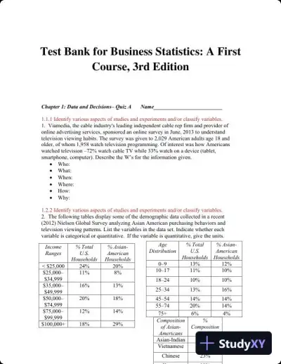 Exam Guides
Test Bank for Business Statistics: A First Course, 3rd Edition
Statistics
436 pages94downloadsFeb 2025 Textbook Guides
Solution Manual for Business Statistics: A First Course, 3rd Edition
Statistics
348 pagesMay 2025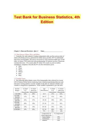 Exam Guides
Test Bank for Business Statistics, 4th Edition
Statistics
714 pagesMay 2025 Exam Guides
Test Bank for Biostatistics for the Biological and Health Sciences , 2nd Edition
Statistics
182 pages161downloadsFeb 2025 Exam Guides
Elementary Statistics, 13th Edition Test Bank
Statistics
239 pages160downloadsFeb 2025 Textbook Guides
Solution Manual For Statistics for Managers Using Microsoft Excel, 7th Edition
Statistics
1418 pages158downloadsFeb 2025 Textbook Guides
Statistics for Managers Using Microsoft Excel 8th Edition Solution Manual
Statistics
1343 pages156downloadsFeb 2025 Textbook Guides
Essentials of Social Statistics for a Diverse Society Second Edition Solution Manual
Statistics
137 pages135downloadsFeb 2025
Study this document with CramX
Once it is in your library, every tool can work from it.