Mathematical Statistics With Applications, 7th Edition Solution Manual

Page 1 of 16

Mathematical Statistics With Applications, 7th Edition Solution Manual - Page 1 preview image

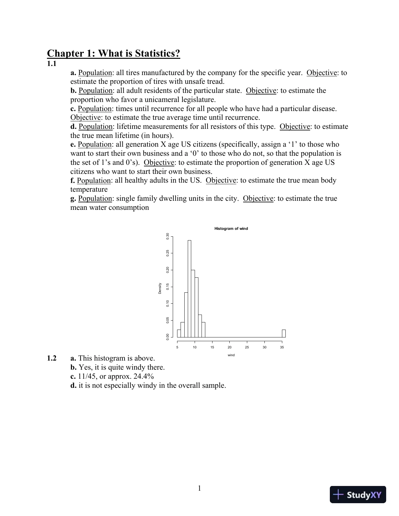
1Chapter 1: What is Statistics?1.1a.Population: all tires manufactured by the company for the specific year. Objective: toestimate the proportion of tires with unsafe tread.b.Population: all adult residents of the particular state. Objective: to estimate theproportion who favor a unicameral legislature.c.Population: times until recurrence for all people who have had a particular disease.Objective: to estimate the true average time until recurrence.d.Population: lifetime measurements for all resistors of this type. Objective: to estimatethe true mean lifetime (in hours).e.Population: all generation X age US citizens (specifically, assign a ‘1’ to those whowant to start their own business and a ‘0’ to those who do not, so that the population isthe set of 1’s and 0’s). Objective: to estimate the proportion of generation X age UScitizens who want to start their own business.f.Population: all healthy adults in the US. Objective: to estimate the true mean bodytemperatureg.Population: single family dwelling units in the city. Objective: to estimate the truemean water consumption1.2a.This histogram is above.Histogram of windwindDensity51015202530350.000.050.100.150.200.250.30b.Yes, it is quite windy there.c.11/45, or approx. 24.4%d.it is not especially windy in the overall sample.

Page 2 of 16

Mathematical Statistics With Applications, 7th Edition Solution Manual - Page 2 preview image

Page 3 of 16

Mathematical Statistics With Applications, 7th Edition Solution Manual - Page 3 preview image

2Chapter 1:What is Statistics?’s Solutions Manual1.3The histogram is above.Histogram of U235U235Density0246810120.000.050.100.150.200.251.4a.The histogram is above.Histogram of stocksstocksDensity246810120.000.050.100.150.200.250.30b.18/40 = 45%c.29/40 = 72.5%1.5a.The categories with the largest grouping of students are 2.45 to 2.65 and 2.65 to 2.85.(both have 7 students).b.7/30c.7/30 + 3/30 + 3/30 + 3/30 = 16/301.6a.The modal category is 2 (quarts of milk). About 36% (9 people) of the 25 are in thiscategory.b..2 + .12 + .04 = .36c.Note that 8% purchased 0 while 4% purchased 5. Thus, 1 – .08 – .04 = .88 purchasedbetween 1 and 4 quarts.

Page 4 of 16

Mathematical Statistics With Applications, 7th Edition Solution Manual - Page 4 preview image

Chapter 1:What is Statistics?3’s Solutions Manual1.7a.There is a possibility of bimodality in the distribution.b.There is a dip in heights at 68 inches.c.If all of the students are roughly the same age, the bimodality could be a result of themen/women distributions.1.8a.The histogram is above.Histogram of AlOAlODensity1012141618200.000.050.100.150.20b.The data appears to be bimodal. Llanederyn and Caldicot have lower sample valuesthan the other two.1.9a.Note that 9.7 = 12 – 2.3 and 14.3 = 12 + 2.3. So, (9.7, 14.3) should containapproximately 68% of the values.b.Note that 7.4 = 12 – 2(2.3) and 16.6 = 12 + 2(2.3). So, (7.4, 16.6) should containapproximately 95% of the values.c.From parts (a) and (b) above, 95% - 68% = 27% lie in both (14.3. 16.6) and (7.4, 9.7).By symmetry, 13.5% should lie in (14.3, 16.6) so that 68% + 13.5% = 81.5% are in (9.7,16.6)d.Since 5.1 and 18.9 represent three standard deviations away from the mean, theproportion outside of these limits is approximately 0.1.10a.14 – 17 = -3.b.Since 68% lie within one standard deviation of the mean, 32% should lie outside. Bysymmetry, 16% should lie below one standard deviation from the mean.c.If normally distributed, approximately 16% of people would spend less than –3 hourson the internet. Since this doesn’t make sense, the population is not normal.1.11a.∑=nic1=c+c+ … +c=nc.b.iniyc∑=1=c(y1+ … +yn) =∑=niiyc1c.()∑=+niiiyx1=x1+y1+x2+y2+ … +xn+yn= (x1+x2+ … +xn) + (y1+y2+ … +yn)

Page 5 of 16

Mathematical Statistics With Applications, 7th Edition Solution Manual - Page 5 preview image

4Chapter 1:What is Statistics?’s Solutions ManualUsing the above, the numerator ofs2is∑=−niiyy12)(=∑=+−niiiyyyy122)2(=∑=−niiy12∑=+niiynyy122Since∑==niiyyn1, we have∑=−niiyy12)(=∑=−niiyny122. Let∑==niiyny11to get the result.1.12Using the data,∑=61iiy= 14 and∑=612iiy= 40. So,s2= (40 - 142/6)/5 = 1.47. So,s= 1.21.1.13a.With∑=451iiy= 440.6 and∑=4512iiy= 5067.38, we have thaty= 9.79 ands= 4.14.b.kintervalfrequencyExp. frequency15.65, 13.934430.621.51, 18.074442.753-2.63, 22.2144451.14a.With∑=251iiy= 80.63 and∑=2512iiy= 500.7459, we have thaty= 3.23 ands= 3.17.b.1.15a.With∑=401iiy= 175.48 and∑=4012iiy= 906.4118, we have thaty= 4.39 ands= 1.87.b.1.16a.Without the extreme value,y= 4.19 ands= 1.44.b.These counts compare more favorably:kintervalfrequencyExp. frequency10.063, 6.39721172-3.104, 9.5642323.753-6.271, 12.7312525kintervalfrequencyExp. frequency12.52, 6.263527.220.65, 8.1339383-1.22, 103940kintervalfrequencyExp. frequency12.75, 5.632526.5221.31, 7.073637.053-0.13, 8.513939

Page 6 of 16

Mathematical Statistics With Applications, 7th Edition Solution Manual - Page 6 preview image

Chapter 1:What is Statistics?5’s Solutions Manual1.17For Ex. 1.2, range/4 = 7.35, whiles= 4.14. For Ex. 1.3, range/4 = 3.04, while = s = 3.17.For Ex. 1.4, range/4 = 2.32, while s = 1.87.1.18The approximation is (800–200)/4 = 150.1.19One standard deviation below the mean is 34 – 53 = –19. The empirical rule suggeststhat 16% of all measurements should lie one standard deviation below the mean. Sincechloroform measurements cannot be negative, this population cannot be normallydistributed.1.20Since approximately 68% will fall between $390 ($420 – $30) to $450 ($420 + $30), theproportion above $450 is approximately 16%.1.21(Similar to exercise 1.20) Having a gain of more than 20 pounds represents allmeasurements greater than one standard deviation below the mean. By the empiricalrule, the proportion above this value is approximately 84%, so the manufacturer isprobably correct.1.22(See exercise 1.11)∑=−niiyy1)(=∑=niiy1–011=−=∑∑==niiniiyyyn.1.23a.(Similar to exercise 1.20) 95 sec = 1 standard deviation above 75 sec, so thispercentage is 16% by the empirical rule.b.(35 sec., 115 sec) represents an interval of 2 standard deviations about the mean, soapproximately 95%c.2 minutes = 120 sec = 2.5 standard deviations above the mean. This is unlikely.1.24a.(112-78)/4 = 8.5b.The histogram is above.Histogram of hrhrFrequency8090100110012345c.With∑=201iiy= 1874.0 and∑=2012iiy= 117,328.0, we have thaty= 93.7 ands= 9.55.

Page 7 of 16

Mathematical Statistics With Applications, 7th Edition Solution Manual - Page 7 preview image

6Chapter 1:What is Statistics?’s Solutions Manuald.1.25a.(716-8)/4 = 177b.The figure is omitted.c.With∑=881iiy= 18,550 and∑=8812iiy= 6,198,356, we have thaty= 210.8 ands= 162.17.d.1.26For Ex. 1.12, 3/1.21 = 2.48. For Ex. 1.24, 34/9.55 = 3.56. For Ex. 1.25, 708/162.17 =4.37. The ratio increases as the sample size increases.1.27(64, 80) is one standard deviation about the mean, so 68% of 340 or approx. 231 scores.(56, 88) is two standard deviations about the mean, so 95% of 340 or 323 scores.1.28(Similar to 1.23) 13 mg/L is one standard deviation below the mean, so 16%.1.29If the empirical rule is assumed, approximately 95% of all bearing should lie in (2.98,3.02) – this interval represents two standard deviations about the mean. So,approximately 5% will lie outside of this interval.1.30Ifμ= 0 andσ= 1.2, we expect 34% to be between 0 and 0 + 1.2 = 1.2. Also,approximately 95%/2 = 47.5% will lie between 0 and 2.4. So, 47.5% – 34% = 13.5%should lie between 1.2 and 2.4.1.31Assuming normality, approximately 95% will lie between 40 and 80 (the standarddeviation is 10). The percent below 40 is approximately 2.5% which is relativelyunlikely.1.32For a sample of sizen, letn′denote the number of measurements that fall outside theintervaly±ks, so that (n–n′)/nis the fraction that falls inside the interval. To show thisfraction is greater than or equal to 1 – 1/k2, note that(n– 1)s2=∑∈−Aiiyy2)(+∑∈−biiyy2)(, (both sums must be positive)whereA= {i: |yi-y|≥ks} andB= {i: |yi–y| <ks}. We have that∑∈−Aiiyy2)(≥∑∈Aisk22=n′k2s2, since ifiis inA, |yi–y|≥ksand there aren′elements inA. Thus, we have thats2≥k2s2n′/(n-1), or 1≥k2n′/(n–1)≥k2n′/n. Thus, 1/k2≥n′/nor(n–n′)/n≥1 – 1/k2.kintervalfrequencyExp. frequency184.1, 103.21313.6274.6, 112.82019365.0, 122.42020kintervalfrequencyExp. frequency148.6, 3736359.842-113.5, 535.18283.63-275.7, 697.38788

Page 8 of 16

Mathematical Statistics With Applications, 7th Edition Solution Manual - Page 8 preview image

Chapter 1:What is Statistics?7’s Solutions Manual1.33Withk=2, at least 1 – 1/4 = 75% should lie within 2 standard deviations of the mean.The interval is (0.5, 10.5).1.34The point 13 is 13 – 5.5 = 7.5 units above the mean, or 7.5/2.5 = 3 standard deviationsabove the mean. By Tchebysheff’s theorem, at least 1 – 1/32= 8/9 will lie within 3standard deviations of the mean. Thus, at most 1/9 of the values will exceed 13.1.35a.(172 – 108)/4 =16b.With∑=151iiy= 2041 and∑=1512iiy= 281,807 we have thaty= 136.1 ands= 17.1c.a= 136.1 – 2(17.1) = 101.9,b= 136.1 + 2(17.1) = 170.3.d.There are 14 observations contained in this interval, and 14/15 = 93.3%. 75% is alower bound.1.36a.The histogram is above.010203040506070ex1.3601234568b.With∑=1001iiy= 66 and∑=10012iiy= 234 we have thaty= 0.66 ands= 1.39.c.Within two standard deviations: 95, within three standard deviations: 96. Thecalculations agree with Tchebysheff’s theorem.1.37Since the lead readings must be non negative, 0 (the smallest possible value) is only 0.33standard deviations from the mean. This indicates that the distribution is skewed.1.38By Tchebysheff’s theorem, at least 3/4 = 75% lie between (0, 140), at least 8/9 liebetween (0, 193), and at least 15/16 lie between (0, 246). The lower bounds are alltruncated a 0 since the measurement cannot be negative.

Page 9 of 16

Mathematical Statistics With Applications, 7th Edition Solution Manual - Page 9 preview image

121Chapter 6: Functions of Random Variables6.1The distribution function ofYis∫−=−=yYyydttyF022)1(2)(, 0≤y≤1.a.2212121211)()(2)()()12()()(1++++−==≤=≤−=≤=uuuYuUFYPuYPuUPuF. Thus,11,)()(2111≤≤−=′=−uuFufuUU.b.22121211212)()(21)()()21()()(2++−−=−==≤=≤−=≤=uuuYuUFYPuYPuUPuF. Thus,11,)()(2122≤≤−=′=+uuFufuUU.c.uuuFuYPuYPuUPuFYU−==≤=≤=≤=2)()()()()(233Thus,10,1)()(133≤≤−=′=uuFufuUU.d..6/1)(,3/1)(,3/1)(321==−=UEUEUEe..6/1)(,3/1)21(,3/1)12(2==−−=−YEYEYE6.2The distribution function ofYis∫−−==yYydttyF132)1)(2/1()2/3()(, –1≤y≤1.a.)118/()3/()3/()3()()(32111−==≤=≤=≤=uuFuYPuYPuUPuFYU. Thus,33,18/)()(211≤≤−=′=uuuFufUU.b.])3(1[)3(1)3()3()()(32122uuFuYPuYPuUPuFYU−−=−−=−≥=≤−=≤=.Thus,42,)3()()(22322≤≤−=′=uuuFufUU.c.2/323)()()()()()(3uuFuFuYuPuYPuUPuFYYU=−−=≤≤−=≤=≤=.Thus,10,)()(2333≤≤=′=uuuFufUU.6.3The distribution function forYis⎪⎩⎪⎨⎧>≤<−≤≤=5.115.112/1102/)(2yyyyyyFY.a.)()()410()()(104104++=≤=≤−=≤=uYuUFYPuYPuUPuF. So,⎪⎩⎪⎨⎧>≤<≤≤−=−+11111664)(101200)4(2uuuuFuuU, and⎪⎩⎪⎨⎧≤<≤≤−=′=+elsewhere011664)()(1011004uuuFufuUU.b.E(U) = 5.583.c.E(10Y– 4) = 10(23/24) – 4 = 5.583.6.4The distribution function ofYis4/1)(yYeyF−−=, 0≤y.a.12/)1(31311)()()13()()(−−−−−==≤=≤+=≤=uuYuUeFYPuYPuUPuF. Thus,1,)()(12/)1(121≥=′=−−ueuFufuUU.b.E(U) = 13.

Page 10 of 16

Mathematical Statistics With Applications, 7th Edition Solution Manual - Page 10 preview image

122Chapter 6: Functions of Random Variables’s Solutions Manual6.5The distribution function ofYis4/)(yyFY=, 1≤y≤5.234123232)()()32()()(−−−==≤=≤+=≤=uuYuUFYPuYPuUPuF. Differentiating,()535,)()(2/123161≤≤=′=−−uuFufuUU.6.6Refer to Ex. 5.10 ad 5.78. Define)()()()(2121uYYPuYYPuUPuFU+≤=≤−=≤=.a.Foru≤0,0)()()(21=≤−=≤=uYYPuUPuFU.For 0≤u< 1,∫ ∫==≤−=≤=+uuyyUudydyuYYPuUPuF02221212/1)()()(22.For 1≤u≤2,∫ ∫−+−−=−=≤−=≤=uuyUudydyuYYPuUPuF202221212/)2(111)()()(2.Thus,⎪⎩⎪⎨⎧≤≤−<≤=′=elsewhere021210)()(yuuuuFufUU.b.E(U) = 1.6.7LetFZ(z) andfZ(z) denote the standard normal distribution and density functionsrespectively.a.).()()()()()(2uFuFuZuPuZPuUPuFZZU−−=≤≤−=≤=≤=Thedensity function forUis then0),()()()()(12121≥=−+=′=uufufufuFufZuZuZuUU.Evaluating, we find0)(2/2/121≥=−−πueuufuU.b.Uhas a gamma distribution withα= 1/2 andβ= 2 (recall thatΓ(1/2) =π).c.This is the chi–square distribution with one degree of freedom.6.8LetFY(y) andfY(y) denote the beta distribution and density functions respectively.a.).1(1)1()1()()(uFuYPuYPuUPuFYU−−=−≥=≤−=≤=The density functionforUis then10,)1()1()()(11)()()(≤≤−=−=′=−α−ββΓαΓβ+αΓuuuufuFufYUU.b.E(U) = 1 –E(Y) =β+αβ.c.V(U) =V(Y).6.9Note that this is the same density from Ex. 5.12:2),(21=yyf, 0≤y1≤1, 0≤y2≤1,0≤y1+y2≤1.a.20021212122)()()()(udydyYuYPuYYPuUPuFuyuU==−≤=≤+=≤=∫ ∫−. Thus,uuFufUU2)()(=′=, 0≤u≤1.b.E(U) = 2/3.c.(found in an earlier exercise in Chapter 5)E(Y1+Y2) = 2/3.

Page 11 of 16

Mathematical Statistics With Applications, 7th Edition Solution Manual - Page 11 preview image

Chapter 6: Functions of Random Variables123’s Solutions Manual6.10Refer to Ex. 5.15 and Ex. 5.108.a.uyuyyUedydyeYuYPuYYPuUPuF−∞+−−==+≤=≤−=≤=∫ ∫1)()()()(0212121221, so thatuUUeuFuf−=′=)()(,u≥0, so thatUhas an exponential distribution withβ= 1.b.From part a above,E(U) = 1.6.11It is given thatfi(yi) =iye−,yi≥0 fori= 1, 2. LetU= (Y1+Y2)/2.a.,21)2()()()(2220221212222121uuuyuyyyYYUueedydyeYuYPuPuUPuF−−−−−+−−==−≤=≤=≤=∫∫so thatuUUueuFuf24)()(−=′=,u≥0, a gamma density withα= 2 andβ= 1/2.b.From part (a),E(U) = 1,V(U) = 1/2.6.12LetFY(y) andfY(y) denote the gamma distribution and density functions respectively.a.)/()()()(cuYPucYPuUPuFU≤=≤=≤=. The density function forUis then0,)/()()(/1))((11≥==′=β−−αβαΓαueucufuFufcucYcUU. Note that this is anothergamma distribution.b.The shape parameter is the same (α), but the scale parameter iscβ.6.13Refer to Ex. 5.8;∫ ∫−−−=−≤=≤+=≤=uyuyyUdydyeYuYPuYYPuUPuF00212121221)()()()(=uuuee−−−−1.Thus,uUUueuFuf−=′=)()(,u≥0.6.14SinceY1andY2are independent, so2221121)(18),(yyyyyf−=, for 0≤y1≤1, 0≤y2≤1.LetU=Y1Y2. Then,∫ ∫−−=>=≤=≤=≤=11/21222112121212)(181)/()/()()()(uyuUdydyyyyYuYPYuYPuYYPuUPuF= 9u2– 8u3+ 6u3lnu.)ln1(18)()(uuuuuFufUU+−=′=, 0≤u≤1.6.15LetUhave a uniform distribution on (0, 1). The distribution function forUisuuUPuFU=≤=)()(, 0≤u≤1. For a functionG, we requireG(U) =YwhereYhasdistribution functionFY(y) =21ye−−,y≥0. Note thatFY(y) =P(Y≤y) =)]([)]([))((11yGFyGUPyUGPU−−=≤=≤=u.So it must be true that=−)(1yG21ye−−=uso thatG(u) = [–ln(1–u)]–1/2. Therefore, therandom variableY= [–ln(U– 1)]–1/2has distribution functionFY(y).

Page 12 of 16

Mathematical Statistics With Applications, 7th Edition Solution Manual - Page 12 preview image

124Chapter 6: Functions of Random Variables’s Solutions Manual6.16Similar to Ex. 6.15. The distribution function forYis.,1)(2bydttbyFybybY≥−==∫−FY(y) =P(Y≤y) =)]([)]([))((11yGFyGUPyUGPU−−=≤=≤=u.So it must be true that=−)(1yGyb−1=uso thatG(u) =ub−1. Therefore, the randomvariableY=b/(1 –U) has distribution functionFY(y).6.17a.Taking the derivative ofF(y),α−αθα=1)(yyf, 0≤y≤θ.b.Following Ex. 6.15 and 6.16, letu=()αθyso thaty=θu1/α. Thus, the random variableY=θU1/αhas distribution functionFY(y).c.From part (b), the transformation isy= 4u. The values are 2.0785, 3.229, 1.5036,1.5610, 2.403.6.18a.Taking the derivative of the distribution function yields1)(−α−ααβ=yyf,y≥β.b.Following Ex. 6.15, let()αβ−=yu1so thatα−β=/1)1(uy. Thus,α−−β=/1)1(UY.c.From part (b),y= 3u−1/. The values are 3.0087, 3.3642, 6.2446, 3.4583, 4.7904.6.19The distribution function forXis:FX(x) =P(X≤x) =P(1/Y≤x) =P(Y≥1/x) = 1 –FY(1/x)= 1 –()[]()ααβ=β−xx1, 0 < x <β–1, which is a power distribution withθ=β–1.6.20a.,)()()()()(2wwFwYPwYPwWPwFYW==≤=≤+≤=0≤w≤1.b.,)()()()()(222wwFwYPwYPwWPwFYW==≤=≤+≤=0≤w≤1.6.21By definition,P(X=i) =P[F(i– 1) <U≤F(i)] =F(i) –F(i– 1), fori= 1, 2, …, since forany 0≤a≤1,P(U≤a) =afor any 0≤a≤1. From Ex. 4.5,P(Y=i) =F(i) –F(i– 1), fori= 1, 2, … . Thus,XandYhave the same distribution.6.22LetUhave a uniform distribution on the interval (0, 1). For a geometric distribution withparameterpand distribution functionF, define the random variableXas:X=kif and only ifF(k– 1) <U≤F(k),k= 1, 2, … .Or sinceF(k) = 1 –qk, we have that:X=kif and only if 1 –qk–1<U≤1 –qk, ORX=kif and only ifqk, < 1–U≤qk–1, ORX=kif and only ifklnq≤ln(1–U)≤(k–1)lnq, ORX=kif and only ifk–1 < [ln(1–U)]/lnq≤k.6.23a.IfU= 2Y– 1, thenY=21+U. Thus,21=dudyand212121)1(2)(uuUuf−+=−=, –1≤u≤1.b.IfU= 1– 2Y, thenY=21U−. Thus,21=dudyand212121)1(2)(uuUuf+−=−=, –1≤u≤1.c.IfU=Y2, thenY=U. Thus,ududy21=anduuuUuuf−=−=121)1(2)(, 0≤u≤1.

Page 13 of 16

Mathematical Statistics With Applications, 7th Edition Solution Manual - Page 13 preview image

Chapter 6: Functions of Random Variables125’s Solutions Manual6.24IfU= 3Y+ 1, thenY=31−U. Thus,31=dudy. With4/41)(yYeyf−=, we have that[]12/)1(12112/)1(4131)(−−−−==uuUeeuf, 1≤u.6.25Refer to Ex. 6.11. The variable of interest isU=221YY+. FixY2=y2. Then,Y1= 2u–y2and21=dudy. The joint density ofUandY2isg(u,y2) = 2e–2u,u≥0,y2≥0, andy2< 2u.Thus,uuuUuedyeuf2202242)(−−==∫foru≥0.6.26a.Using the transformation approach,Y=U1/mso thatmmmdudyu/)1(1−−=so that the densityfunction forUisα−α=/1)(uUeuf,u≥0. Note that this is the exponential distributionwith meanα.b.∫∞α−α==0/1//)()(dueuUEYEumkmkk=()mkmk/1α+Γ, using the result from Ex. 4.111.6.27a.LetW=Y. The random variableYis exponential soβ−β=/1)(yYeyf. Then,Y=W2andwdwdy2=. Then,β−β=/22)(wYweyf,w≥0, which is Weibull withm= 2.b.It follows from Ex. 6.26 thatE(Yk/2) =()2/21kkβ+Γ6.28IfYis uniform on the interval (0, 1),1)(=ufU. Then,2/UeY−=and2/21ududye−−=.Then,2/212/21||1)(uuYeeyf−−=−=,u≥0 which is exponential with mean 2.6.29a.With22mVW=,mWV2=andmwdwdv21||=. Then,kTwmambwmwmwaWewewf/2/12/22)/2(2/3)(−−==,w≥0.The above expression is in the form of a gamma density, so the constantamust bechosen so that the density integrate to 1, or simply2/3232/3))((12kTmaΓ=.So, the density function forWiskTwkTWewwf/2/1))((12/323)(−Γ=.b.For a gamma random variable,E(W) =kT23.6.30The density function forIis2/1)(=ifI, 9≤i≤11. ForP= 2I2,I=2/Pand2/12/3)2/1(−=pdpdi. Then,pppf241)(=, 162≤p≤242.

Page 14 of 16

Mathematical Statistics With Applications, 7th Edition Solution Manual - Page 14 preview image

126Chapter 6: Functions of Random Variables’s Solutions Manual6.31Similar to Ex. 6.25. FixY1=y1. Then,U=Y2/y1,Y2=y1Uand1||2ydudy=. The jointdensity ofY1andUis2/)1(218111),(uyeyuyf+−=,y1≥0,u≥0. So, the marginaldensity forUis31)1(2012/)1(2181)(uuyUdyeyuf+∞+−==∫,u≥0.6.32NowfY(y) = 1/4, 1≤y≤5. IfU= 2Y2+ 3, thenY=()2/123−Uand()3241||−=ududy. Thus,)3(281)(−=uUuf, 5≤u≤53.6.33IfU= 5 – (Y/2),Y= 2(5 –U). Thus,2||=dudyand)33180(4)(2uuufU+−=, 4.5≤u≤5.6.34a.IfU=Y2,Y=U. Thus,ududy21||=andθ−θ=/1)(uUeuf,u≥0. This is theexponential density with meanθ.b.From part a,E(Y) =E(U1/2) =2πθ. Also,E(Y2) =E(U) =θ, soV(Y) =]1[4π−θ.6.35By independence,1),(21=yyf, 0≤y1≤0, 0≤y2≤1. LetU=Y1Y2. For a fixed valueofY1aty1, theny2=u/y1. So that121ydudy=. So, the joint density ofY1andUis11/1),(yuyg=, 0≤y1≤0, 0≤u≤y1.Thus,)ln()/1()(111udyyufuU−==∫, 0≤u≤1.6.36By independence,)(4212221221),(yyyyeyyf+−θ=,y1> 0,y2> 0. LetU=2221YY+. For a fixedvalue ofY1aty1, thenU=2221Yy+so we can write212yuy−=. Then,21221yududy−=sothat the joint density ofY1andUis21221121/41),(yuuyuyeuyg−θ−θ−==θ−θ/122uey, for 0 <y1<u.Then,θ−θθ−θ==∫/110/1222)(uuuUuedyeyuf. Thus,Uhas a gamma distribution withα= 2.6.37The mass function for the Bernoulli distribution isyyppyp−−=1)1()(,y= 0, 1.a.txtytYYpepypeeEtm+−===∑=1)()()(1011.b.ntniYtWWpeptmeEtmi]1[)()()(1+−===∏=c.Since the mgf forWis in the form of a binomial mgf withntrials and successprobabilityp, this is the distribution forW.

Page 15 of 16

Mathematical Statistics With Applications, 7th Edition Solution Manual - Page 15 preview image

Chapter 6: Functions of Random Variables127’s Solutions Manual6.38LetY1andY2have mgfs as given, and letU=a1Y1+a2Y2. The mdf forUis)()()()()()()(21)()()(2122112211tamtameEeEeEeEtmYYYtaYtatYaYaUtU====+.6.39The mgf for the exponential distribution withβ= 1 is1)1()(−−=ttm,t< 1. Thus, withY1andY2each having this distribution andU= (Y1+Y2)/2. Using the result from Ex.6.38, leta1=a2= 1/2 so the mgf forUis.)2/1()2/()2/()(2−−==ttmtmtmUNote thatthis is the mgf for a gamma random variable withα= 2,β= 1/2, so the density functionforUis0,4)(2≥=−uueufuU.6.40It has been shown that the distribution of both21Yand22Yis chi–square withν= 1. Thus,both have mgf2/1)21()(−−=ttm,t< 1/2. WithU=21Y+22Y, use the result from Ex.6.38 witha1=a2= 1 so that.)21()()()(1−−==ttmtmtmUNote that this is the mgf for aexponential random variable withβ= 2, so the density function forUis0,)(2/21≥=−ueufuU(this is also the chi–square distribution withν= 2.)6.41(Special case of Theorem 6.3) The mgf for the normal distribution with parametersμandσis2/22)(ttetmσ+μ=. Since theYi’s are independent, the mgf forUis given by[]∑∑∏∏σ+μ======iiiniinitYaUtUiiiatattameEeEtm22211)2/(exp)()()()(.This is the mgf for a normal variable with mean∑μiiaand variance∑σiia22.6.42The probability of interest isP(Y2>Y1) =P(Y2–Y1> 0). By Theorem 6.3, thedistribution ofY2–Y1is normal withμ= 4000 – 5000 = –1000 andσ2= 4002+ 3002=250,000. Thus,P(Y2–Y1> 0) =P(Z>000,250)1000(0−−) =P(Z> 2) = .0228.6.43a.From Ex. 6.41,Yhas a normal distribution with meanμand varianceσ2/n.b.For the given values,Yhas a normal distribution with varianceσ2/n= 16/25. Thus,the standard deviation is 4/5 so thatP(|Y–μ|≤1) =P(–1≤Y–μ≤1) =P(–1.25≤Z≤1.25) = .7888.c.Similar to the above, the probabilities are .8664, .9544, .9756. So, as the sample sizeincreases, so does the probability thatP(|Y–μ|≤1).6.44The total weight of the watermelons in the packing container is given by∑==niiYU1, soby Theorem 6.3Uhas a normal distribution with mean 15nand variance 4n. We requirethat)()140(05.415140nnZPUP−>=>=. Thus,nn415140−=z.05= 1.645. Solving thisnonlinear expression forn, we see thatn≈8.687. Therefore, the maximum number ofwatermelons that should be put in the container is 8 (note that with this valuen, we haveP(U> 140) = .0002).

Page 16 of 16

Mathematical Statistics With Applications, 7th Edition Solution Manual - Page 16 preview image

128Chapter 6: Functions of Random Variables’s Solutions Manual6.45By Theorem 6.3 we have thatU= 100 +7Y1+ 3Y2is a normal random variable with meanμ= 100 + 7(10) + 3(4) = 182 and varianceσ2= 49(.5)2+ 9(.2)2= 12.61. We require avaluecsuch thatP(U>c) =P(61.12182−>cZ). So,61.12182−c= 2.33 andc= $190.27.6.46The mgf for W is2/)/2()21()/2()()()(nYtYWtWttmeEeEtm−β−=β===. This is the mgffor a chi–square variable withndegrees of freedom.6.47By Ex. 6.46,U= 2Y/4.2 has a chi–square distribution withν= 7. So, by Table III,P(Y> 33.627) =P(U> 2(33.627)/4.2) =P(U> 16.0128) = .025.6.48From Ex. 6.40, we know thatV=21Y+22Yhas a chi–square distribution withν= 2. Thedensity function forVis2/21)(vVevf−=,v≥0. The distribution function ofU=Vis)()()()(22uFuVPuUPuFVU=≤=≤=, so that2/2)()(uUUueuFuf−=′=,u≥0. A sharpobserver would note that this is a Weibull density with shape parameter 2 and scale 2.6.49The mgfs forY1andY2are, respectively,11]1[)(ntYpeptm+−=,22]1[)(ntYpeptm+−=.SinceY1andY2are independent, the mgf forY1+Y2is2121]1[)()(nntYYpeptmtm++−=×.This is the mgf of a binomial withn1+n2trials and success probabilityp.6.50The mgf forYisntYpeptm]1[)(+−=. Now, defineX=n–Y. The mgf forXisntYtnYnttXXepptmeeEeEtm])1([)()()()()(−+=−===−.This is an mgf for a binomial withntrials and “success” probability (1 –p). Note that therandom variableX= # offailuresobserved in the experiment.6.51From Ex. 6.50, the distribution ofn2–Y2is binomial withn2trials and “success”probability 1 – .8 = .2. Thus, by Ex. 6.49, the distribution ofY1+ (n2–Y2) is binomialwithn1+n2trials and success probabilityp= .2.6.52The mgfs forY1andY2are, respectively,)1(11)(−λ=teYetm,)1(22)(−λ=teYetm.a.SinceY1andY2are independent, the mgf forY1+Y2is)1)((2121)()(−λ+λ=×teYYetmtm.This is the mgf of a Poisson with meanλ1+λ2.b.From Ex. 5.39, the distribution is binomial withmtrials andp=211λ+λλ.6.53The mgf for a binomial variableYiwithnitrials and success probabilitypiis given byiintiiYepptm]1[)(+−=. Thus, the mgf for∑==niiYU1∏+−=intiiUiepptm]1[)(is.a.Letpi=pandni=mfor alli. Here,Uis binomial withm(n) trials and successprobabilityp.b.Letpi=p. Here,Uis binomial with∑=niin1trials and success probabilityp.c.(Similar to Ex. 5.40) The cond. distribution is hypergeometric w/r=ni,N=∑in.d.By definition,

Preview Mode

This document has 334 pages. Sign in to access the full document!

Report

Learning Tools

Writing Tools

Browse Resources

Mathematical Statistics With Applications, 7th Edition Solution Manual - Page 1

Study Now!

Document Details

Related Documents

Statistics - Univariate Inferential Tests

Statistics - Sampling

Statistics - Probability

Statistics - Principles of Testing

Statistics - Numerical Measures

Statistics - Introduction to Statistics

Statistics - Graphic Displays

Statistics - Cummulative Reviews

Statistics - Common Mistakes and Tables

Statistics - Bivariate Relationships

Company

Explore

Study Tools