

Social Statistics for a Diverse Society Eighth Edition Solution Manual
- Statistics
- 93 pages
- Shared May 2025
Social Statistics for a Diverse Society Eighth Edition Solution Manual is your study companion, providing answers to textbook exercises and reinforcing key concepts.
Preview 16 of 93 pages
See the first 16 pages exactly as they appear in the document.
Page 1 Read page 1 as text
CHAPTER 1— ANSWERS TO EXERCISES 1. Once our research question, the hypothesis, and the study variables have been selected, we move on to the next stage of the research process—measuring and collecting the data. The choice of a particular data collection method or instrument depends on our study objective. After our data have been collected, we have to find a systematic way to organize and analyze our data and set up some set of procedures to decide what we mean. 2. a. Democrats and Independents are more likely to support the Affordable Care Act than Republicans. b. Whites have greater incomes than any other race. Hispanics have incomes greater than blacks but less than whites. c. As the number of police in a city increases, the crime rate will decrease. d. Life satisfaction may vary with marital status, with satisfaction higher among married per - sons than those not married. e. Younger adults are more likely to support the legalization of marijuana than older adults. f. Ethnic minority families are more likely to arrange in-home care (vs. formal institutional care) for their elderly parents than nonminority families. 3. a. Interval-ratio b. Interval-ratio c. Nominal d. Ordinal e. Nominal f. Interval-ratio g. Ordinal 4. a. Discrete b. Continuous f. Continuous 5. There are many possible variables from which to choose. Some of the most common selections by students will probably be as follows: type of occupation or industry, work experience, and educational training or expertise. Students should first address the relationship between these variables and gender. Students may also consider measuring structural bias or discrimination.
Page 2 Page 3 Read page 3 as text
6. a. Unemployment records could be used to determine the actual number of unemployed; a descriptive statistic based on the population. b. A survey is taken to estimate student opinions about the quality of food; inferential statistic. c. National health records can be used to determine the incidence rate of breast cancer among all Asian women, so this would be a descriptive statistic. d. The ratings will be gathered from a survey, so this is inferential. e. A university should be able to report GPA by major, so this is a descriptive statistic based on the population. f. In theory, the United States records all immigrants to this country. Therefore, the number of South East Asian immigrants would be a descriptive statistic. However, because of illegal immigration, surveys are also taken to estimate the total number of legal and unauthorized immigrants. In that event, the number of immigrants would be an inferential statistic. 7. a. Annual income b. Gender—nominal; Number of hours worked per week—interval-ratio; Years of education— interval-ratio; Job title—nominal. c. This is an application of inferential statistics. She is using information based on her sample to predict the annual income of a larger population of young graduates. 8. At the nominal level, a simple measure of political participation is whether or not someone voted in the most recent general election. This variable would be coded either “ yes” or “ no.” At the ordinal level, a composite measure could be constructed of both voting and political party membership, like this: Behavior Code Didn’t vote, no membership 0 Voted, no membership OR Membership, didn’t vote 1 Voted and membership 2 These codes are ordinal in scale because the amount of political participation can be ranked from high to low. Other possible ordinal variables can be constructed from other sets of behaviors, such as working in a candidate’s campaign, signing a petition, and so forth. The key points are to create a variable whose values can be ranked and whose values are not on an interval-ratio scale. At the interval-ratio level, political participation could be measured by the percentage of elec - tions in which a person has voted since becoming eligible to vote or the amount of money a person donated to political candidates during some specified time period. 9. a. Individual age: This variable could be measured as an interval-ratio variable, with actual age in years reported. As discussed in the chapter, interval-ratio variables are the highest level of measurement and can also be measured at ordinal or nominal levels.
Page 4 Read page 4 as text
b. Annual income: This variable could be measured as an interval-ratio variable, with actual dollar earnings reported. c. Religiosity: This variable could be measured in several ways. For example, as church attendance, the variable could be ordinal (number of times attended church in a month: every week, at least twice a month, less than two times a month, none at all). d. Student performance: This could be measured as an interval-ratio variable as GPA or test score. e. Social class: This variable is an ordinal variable, with categories low, working, middle, and upper. f. Number of children: This variable could be measured in several ways. As an interval-ratio measure, the actual number of children could be reported. As an ordinal measure, the number of children could be measured in categories: 0, 1–2, 3–4, 5 or more. This could also be a nominal measurement—do you have children? Yes or No.
Page 5 Read page 5 as text
CHAPTER 2— ANSWERS TO EXERCISES 1. a. Race is a nominal variable. Class is an ordinal variable, since the categories can be ordered. Trauma is an interval variable. b. Frequency Table for Race Race Frequency (f) White 17 Nonwhite 13 Total ( N ) 30 c. White: 17/30 = .57%; Nonwhite: 13/30 = .43 2. Frequency and Percentage Distribution Table for Class Class Frequency (f) Percentage (%) Lower 3 10 Working 15 50 Middle 11 36.7 Upper 1 3.3 Total ( N ) 30 100 a. The smallest perceived class group is the upper class, composing only 3.3% of the survey. b. Together, the working and middle class compose 86.7% of the survey. 3. Number of Traumas Frequency (f) 0 15 1 11 2 4 Total ( N ) 30 a. Trauma is an interval or ratio-level variable, since it has a real zero point and a meaningful numeric scale. b. People in this survey are more likely to have experienced no traumas last year (50% of the group).
Page 6 Read page 6 as text
c. The proportion who experienced one or more traumas is calculated by first adding 36.7% and 13.3% = 50%. Then, divide that number by 100 to obtain the proportion, 0.50, or half the group. 4. We use pie charts to visually present these data. Nonwhite 43% White 57% Lower 10% Upper 3% Working 50% Middle 37% 5. Support does vary by political party. The majority of strong Democrats (58.1%) and Independents (66%) agree/strongly agree with the statement. The group with the lowest percentage of agreement is Strong Republicans at 49%. The percentage disagreeing with the statement is highest among Strong Republicans (36.7%) compared with 12.3% of Strong Democrats and 11.3% of Independents. 6. a. E-mail Hours per Week Frequency Cumulative Frequency Percentage (%) Cumulative Percentage (C%) 0 19 19 19 19 1 20 39 20 39 2 13 52 13 52 3 5 57 5 57 4 2 59 2 59 5 6 65 6 65 6 5 70 5 70 No traumas 50% 1 trauma 37% 2 traumas 13%
Page 7 Read page 7 as text
E-mail Hours per Week Frequency Cumulative Frequency Percentage (%) Cumulative Percentage (C%) 7 2 72 2 72 8 3 75 3 75 9 1 76 1 76 10 or more 23 99 23 99 Total 99 99% b. .575 ( 57/ 99) spent 3 hours or less on e-mail per week. c. This group includes 5 + 2 + 3 + 1 + 23 = 34 respondents. The proportion is 34/99 or .343. d. This is an interval-ratio variable. The appropriate graphic presentation would be either a histogram or a line graph. 7. The group with the largest increase in voting rates is blacks, from 53% in 1996 to 66.2% in 2012. Blacks are the only group that did not experience a decline in voting rates for the years presented. Hispanic voting rates exceeded the voting rates for Asians in 2000 and remained higher than Asians through 2012. Hispanics and Asians have the lowest voting rates for all groups. As noted in the exercise, in the 2012 presidential election, blacks had the highest voting rates for all groups, followed by non-Hispanic whites, Hispanics, and Asians. White voting rates declined by 2% from 2008 to 2012. The highest voting rate for whites was in 2004 (67.2%), in 2008 for Hispanics (49.9%) and for Asians (47.6%). 8. From 1970 to 2013, European immigrants had the highest increase in the percentage who completed at least high school (95 − 48 = 47%). During the same time period, immigrants from the Caribbean had the second highest increase (72 − 36 = 36%). Since 1970 at least 50% of immigrants from Other Central/South America countries, Asia, and Africa had achieved at least a high school education. In 2013, at least 66% of immigrants from five out of the six reported regions achieved a high school education. Throughout all the years reported in the table, immigrants from Mexico have the lowest percentage of high school completion. 9. If we identify younger Americans as those in the 18 to 24 and 25 to 44 age-groups and older Americans in the 45–64, 65–74, and 75 and over categories—the data indicate that as age increases, so does the percentage voting in a Presidential election. The group with the high - est percentage of voting is the 65- to 74-year olds, with 73.5% voting. The percentage drops for the 75 and over age-group, but is still higher than the reported percentages for the age- groups: 18–24, 25–44, and 45–64. 10. Please note: The data are as reported by the Bureau of Justice Statistics. The percentages do not add up to 100%. All Males (%) Cumulative Percentage (C%) All Females (%) Cumulative Percentage (C%) 18–19 1 1 .6 .6 20–24 11.4 12.4 10 10.6 25–29 15.4 27.8 17.5 28.1 30–34 16.5 44.3 18.6 46.7 35–39 14.2 58.5 14.7 61.4 (Continued)
Page 8 Read page 8 as text
All Males (%) Cumulative Percentage (C%) All Females (%) Cumulative Percentage (C%) 40–44 12.2 70.7 12.8 74.2 45–49 10.4 81.1 10.9 85.1 50–54 8.5 89.6 7.7 92.8 55–59 5.2 94.8 3.9 96.7 60–64 2.7 97.5 1.8 98.5 65 + 2.3 99.8 1.2 99.7 11. Overall, the highest percentage of smokers are in the 12th-grade category; the lowest are stu - dents in the 8th grade. The highest percentage of daily smokers for all grades is between 1996 and 1997 with percentages declining through 2014. (There are no data for 8th and 10th graders pre-1990.) Since 2012, the percentage of students smoking daily was at 10% or below. 12. For all racial and Hispanic groups presented in the bar graph, the percentage of uninsured individuals decreased from 2013 to 2014. Hispanics have the highest percentage of unin - sured, followed by blacks, Asians, and whites. According to these data, in 2014, more than a 1/3 of Hispanics did not have health insurance. The group with the largest decline is non- Hispanic blacks (24.7 − 17.6 = 7.1%); the smallest reduction is among non-Hispanic whites (14.5 − 11.5 = 3.0%). 13. a. For Africa, Asia, Oceania, and Latin America, the largest age-group is 18 to 44 years. For Europe and North America, the age composition is slightly older; individuals aged 45 to 64 years are the largest age-group for both. b. We display the data in a vertical bar graph. We selected a bar graph because country of origin (the basis of the percentage calculation) is nominal. 0 10 20 30 40 50 60 Africa Asia Europe North America Oceania Latin America 65 + 45–64 18–44 under 18 (Continued)
Page 9 Read page 9 as text
SPSS SOLUTIONS 1. a. The valid number of responses is 990. b. 22.3% reported being in excellent health; 7.0% in poor health. c. HEALTH is an ordinal measure. The best way to graphically present it would be in a bar graph. 2. a.
Page 10 Read page 10 as text
b. Each variable is an ordinal measurement. The higher value (5) indicates strong disagree - ment with the statement (though the label does not appear in our screenshots). Overall, respondents express positive attitudes toward immigrants. Most believe that immigrants should have the same education as Americans (19.8 + 67.4 = 87.2% agree or strongly agree to the statement), disagree that immigrants undermine American culture (49.1 + 8.9 = 58% disagree or strongly disagree ), and disagree that immigrants take away jobs (35 + 6.6 = 41.6% disagree or strongly disagree ). 3.
Page 11 Read page 11 as text
a. GOODLIFE is an ordinal measure (a 5-point scale). b. GOODLIFE may vary by respondent’s age, social class, employment status, education, and one’s overall happiness with life. You may want to explore the relationship between GOODLIFE and these variables on your own using the GSS data sets. c. This is an ordinal measure and should be presented as a bar graph. 4. Students are encouraged to determine on their own how to recode the variable. Students should consider how the years of education indicates attainment of a specific degree, for example: 12 years = high school graduate or 16 years = college graduate. 5. a. Nominal, as a pie chart or bar graph. b. Interval measure, as a histogram or line chart. c. Ordinal measure, as a bar graph. d. Interval measure, as a histogram or line chart.
Page 12 Read page 12 as text
CHAPTER 3— ANSWERS TO EXERCISES 1. a. Mode = Routine ( f = 379) b. Median = Routine c. Based on the mode and median for this variable, most respondents indicate that their lives are “routine.” d. A mean score could not be interpreted for this variable. A mean would have no meaning for a nominal measurement. 2. a. Ordinal. b. The mode can be found in two ways: by looking for the (1) highest frequency ( f = 251) or (2) highest percentage (32.5%)—“strongly agree”. c. The median can be found in two ways: by using either the frequencies column or the cumulative percentages. Using Frequencies Using Cumulative Percentages N + = + = 1 2 1 2 387th case 773 Notice that 50% of the observations fall in the “agree” cumulative percentage category. Starting with the frequency in the first category (251), add up the frequencies until you find where the 387th case falls.The 387th case falls at the “agree” category, which is the median. The 50% mark, or the median, is located in the “agree” category. The data indicate strong support for same-sex marriage. The largest single category is “strongly agree”— 32.5%. Combined with the “agree” category (the second largest category), more than half of the GSS sample agree that homosexuals should have the right to marry (32.5 + 25.2 = 57.7). 3. a. Interval ratio. The mode can be found in two ways: by looking either for the highest frequency (14) or the highest percentage (43.8%). The mode is the category that corre - sponds to the value “40 hours worked last week.” The median can be found in two ways: by using either the frequencies column or the cumulative percentages.
Page 13 Read page 13 as text
Using Frequencies Using Cumulative Percentages N + = + = 1 2 1 2 th case 32 16 5 . Notice that 34.4% of the observations fall in or below the “32 hours worked last week” category; 78.1% fall in or below the “40 hours worked last week” category. Starting with the frequency in the first category (1), add up the frequencies until you find where the 16th and 17th cases fall. Both these cases correspond to the category “40 hours worked last week,” which is the median. The 50% mark, or the median, is located somewhere within the “40 hours worked last week” category. So the median is “40 hours worked last week.” b. Since the median is merely a synonym for the 50th percentile, we already know that its value is “40 hours worked last week.” 25th percentile = (32 × 0.25) = 8th case = 30 hours worked last week. 75th percentile = (32 × 0.75) = 24th case = 40 hours worked last week 4. a. The mode category is “very important”, f = 136. b. The median can be found in two ways: either by using the frequencies column or by cal - culating the cumulative percentages. The median score is 3—not very important. c. 20th percentile = (392 × 0.20) = 78th case = “Very important” 80th percentile = (392 × 0.80) = 314th case = “Not important at all”
Page 14 Read page 14 as text
5. a. Mode Median Black Seldom ( f = 11) Sometimes White Everyday ( f = 84) Nearly everyday Hispanic Everday ( f = 25) Most days b. Teens’ breakfast habits vary by race/ethnicity. Out of the three racial/ethnic groups, black students were more likely to report seldom or sometimes eating breakfast. On the other hand, white and Hispanic students eat breakfast more frequently. The mode for white and Hispanic students is everyday. 6. The mode can be found by looking for the highest frequency in each column; the mode for each group is listed below: Males: Working full time Females: Working full time The median can be found in two ways: either by using the frequencies column or by using the cumulative percentages. However, since the problem only gives the frequencies, we’ll use those to solve for the median.
Page 15 Read page 15 as text
Males Females N + = + = 1 2 1 2 th case 513 257 N + = + = 1 2 1 2 nd case 503 252 Starting with the frequency in the first category (303), add up the frequencies until you find where the 257th case falls. We actually don’t need to do any adding, as both these cases correspond with the first category, “Working Full Time.” Starting with the frequency in the first category (263), add up the frequencies until you find where the 252nd case falls. We actually don’t need to do any adding, as both these cases correspond with the first category, “Working Full Time.” When using both the mode and the median to estimate participation in the labor force, it appears that there are no substantial differences between males and females. 7. We begin by multiplying each household size by its frequency. Household Size Frequency Frequency × Y(f Y) 1 381 381 2 526 1,052 3 227 681 4 200 800 5 96 480 6 42 252 7 19 133 8 5 40 9 2 18 10 2 20 Total N = 1,500 ∑ fY = 3,857 Y f Y N = = = Σ 3,857 1,500 2.57 The mean number of people per household is 2.57. 8. a. Based on the table, the 90th percentile is in response category “4.” b. The median is “2.” c. The mean is 2.46 = 1,673/679. d. The distribution is slightly positively skewed; the mean is larger than the median.
Page 16 Read page 16 as text
Ideal Number of Children Frequency Frequency × Y(fY) 0 11 0 1 14 14 2 395 790 3 188 564 4 56 224 5 11 55 6 2 12 7 2 14 Total N = 679 ∑ fY = 1,673 9. a. There appear to be a few outliers (i.e., extremely high values); this leads us to believe that the distribution is skewed in the positive direction. 0 0 100 200 300 400 500 600 2 4 6 8 Number of Persons in Household Frequency 10 12 b. The median can be found in two ways: by using either the frequencies column or the cumulative percentages. The data are in frequencies; we’ll use those to solve the median. Because the median (2) is less than the mean (2.57), we can conclude that the distribution is skewed in a positive direction. Our answer to Question 9a is further supported.
77 more pages in the full document
Unlock it once and it stays in your library, ready to chat with or turn into flashcards.
Unlock the full documentMore Statistics study materials
See all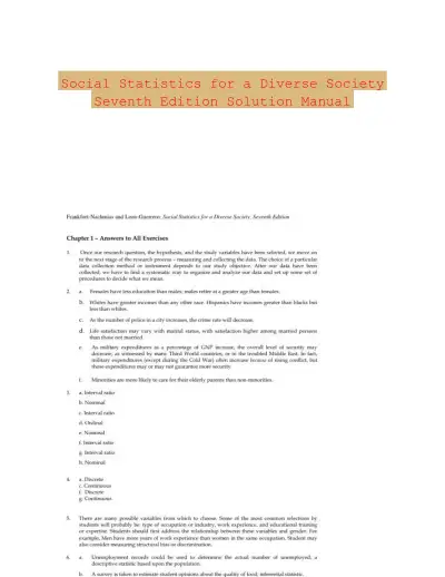 Textbook Guides
Social Statistics for a Diverse Society Seventh Edition Solution Manual
Statistics
88 pagesMay 2025 Exam Guides
Test Bank for Biostatistics for the Biological and Health Sciences , 2nd Edition
Statistics
182 pages161downloadsFeb 2025 Exam Guides
Elementary Statistics, 13th Edition Test Bank
Statistics
239 pages160downloadsFeb 2025 Textbook Guides
Solution Manual For Statistics for Managers Using Microsoft Excel, 7th Edition
Statistics
1418 pages158downloadsFeb 2025 Textbook Guides
Statistics for Managers Using Microsoft Excel 8th Edition Solution Manual
Statistics
1343 pages156downloadsFeb 2025 Textbook Guides
Essentials of Social Statistics for a Diverse Society Second Edition Solution Manual
Statistics
137 pages135downloadsFeb 2025 Exam Guides
Test Bank For Elementary Statistics, 3rd Edition
Statistics
969 pages126downloadsFeb 2025 Textbook Guides
Solution Manual for Business Statistics, 4th Edition
Statistics
582 pages125downloadsFeb 2025
Study this document with CramX
Once it is in your library, every tool can work from it.