

STAT 501 Mid-Term Exam 2 Spring 2015
- Statistics
- Pennsylvania State University
- 11 pages
- Shared May 2025
A mid-term exam assessing statistical analysis and hypothesis testing.
Preview 4 of 11 pages
See the first 4 pages exactly as they appear in the document.
Page 1 Read page 1 as text
STAT 501 – Mid - Term Exam 2 – Spring 2015 – Due April 12 Instructions : Use Word to type your answers within this document. Then, submit your answers in the appropriate dropbox in ANGEL by the due date and within 3 hours of downloading the exam . The point distribution is located next to each question. 1. ( 4 x2 = 8 points) State which of the following statements is TRUE and which is FALSE. For the statements that are false , explain why they are false . a. R emov ing an outlier in a regression analysis will result in narrower confidence interval s . b. In a simple linear regression (SLR) model, if a log transformation is performed on X to remedy some non - linearity, the mean value of Y is bound to change. c. In model selection, t he high e st adjusted R 2 - value and the smallest S - value criteria always yield the same "best" models. d. Regression models with different r esponses, but the same predictor X matrix, will have the same leverage values. 2. (3+3+4+4+3+3 = 20 points) Open the “ Salary Data . ” The data set consis t s of current salaries (Salary in thousands of dollars ) fo r 63 individuals with information about their years of work experience ( YrsExp ) and highest degree attained (Degree) . Your goal is to fit a regression model to express the dependence of Y ( Salary ) on X ( YrsExp ) and Degree . a. Clearly d efine a set of indicator variables that could be used in a regression model to represent the qualitative variable Degree . [Hint: T hink carefully about the number of indicator variables needed given the number of levels of Degree and use “Bachelor” as the reference level. ] b. Write a population multiple linear regression equation for predictin g the current salary in terms of YrsExp and Degree . Since education leve l could impact th e dependence of Y on X, t he model should contain an interaction ef fect between YrsExp and Degree , together with their main effects. [Hint: Yo ur equation should include Y, X, the indicator variables you defined in part (a) , interaction terms, and population regression coefficients ( β ’s). ] c. Conduct a hypothesis t est for whether the average annual salary increase per year of experience differs by level of education (i.e., test if the slopes for two or more Degree categories differ ) . Write out the null and alternative hypotheses, the test statistic, the p - value, and the conclusion. [Minitab v17: Select S alary as the Response, YrsExp as the Continuous predictor , Degree as the categorical predictor, click “Model,” select both YrsExp and Degree together in the Predictors box and click the Add button next to “Interactions through order 2 . ” Minitab v16: Create interaction terms using Calc > Calculator before fitting the regression model. ] d. Write a new population regression equation based on your conclusion to part (c). Fit this model and conduct two separate hypothesis t est s for whether the mean salary for a fixed number of years’ experience differs by education level . For each test, write out the null and alternative hypotheses, the test statistic, the p - value, and the conclusion.
Page 2 Page 3 Read page 3 as text
e. Based on your conclusion to part (d) , write th r e e fitted sample regression equation s that can be used to predict the current salary for each education level . [Hint: Y our equations should include number values, not β ’s. ] f. Based on one of the equation s from part (e), p redict the current salary of a PhD degree holder with 10 year s of work experience . [Hint: A point estimate is sufficient so there is no need for an interval .] 3. (4x2 = 8 points) Consider the following four graphs where the vertical axis represents Y and the horizontal axis represents X. Choose the most appropriate plot for each of the following models (where D 1 and D 2 represent a set of indicator variables) : a. 𝐸 ( 𝑌 ) = 𝛽 0 + 𝛽 1 𝑋 b. 𝐸 ( 𝑌 ) = 𝛽 0 + 𝛽 1 𝑋 + 𝛽 4 𝐷 1 𝑋 + 𝛽 5 𝐷 2 𝑋 c. 𝐸 ( 𝑌 ) = 𝛽 0 + 𝛽 1 𝑋 + 𝛽 2 𝐷 1 + 𝛽 3 𝐷 2 d. 𝐸 ( 𝑌 ) = 𝛽 0 + 𝛽 1 𝑋 + 𝛽 2 𝐷 1 + 𝛽 3 𝐷 2 + 𝛽 4 𝐷 1 𝑋
Page 4 Read page 4 as text
4. ( 5+2+5+3+3 = 18 points) The file “ Savings Data ” contains savings of 33 individuals along with their age . It is apparent that Y = S avings (in $) has a positive association with X = A ge (in years) . An appropriate regression model relating S avings to A ge could be useful for predicting savings based on age. The most straightforward approach would be to fit a simple linear regression (SLR) model for Y vs X, provided that the LINE assumptions are satisfied. [Consult “Worked Examples Using Minitab” in the Online Notes for help with any Minitab procedures.] a. Fit an SLR model for Y vs X and p erform a residual plot analysis to determine if the LINE assumptions are satisfied. Include a numerical test when checking for normality (u se t he Ryan Joiner test in Minitab). Discuss your findings and include any relevant graphs. b. Based on your conclusion in part ( a ) , determine if any transformations are suggested for X and/or Y. [Hint: You should find that both X and Y need to be transformed.] c. Fit an SLR model for the transformed variable ( s ) and comment on this model’s validity with supporting statements, numerical tests and/or plots . d. Use Minitab to compute a 95% confidence interval for the mean amount of savings (in $) expected for 40 year - olds based on the fitted model in part ( c ) . [Hint: R emember to take into account the transformations to X and Y.] e. Use Minitab to compute a 95% prediction interval for the amount of savings (in $) predicted for a randomly selected 40 year - old based on the fitted model in part ( c ) . [Hint: R emember to take into account the transformations to X and Y.] 5. (2+1+3+2 = 8 points) The following Minitab output resulted from a multiple linear regression model fit to response variable, Y , and predictor terms, X 1 , X 2 , and X 1 X 2 : Coefficients Term Coef SE Coef T - Value P - Value Constant 4.49 1.89 2.37 0.022 X1 0.759 0.374 2.03 0.048 X2 0.965 0.426 2.26 0.028 X1*X2 0.1742 0.0821 2.12 0.039 a. Conduct a hypothesis test for whether the interaction term, X 1 X 2 , can be dropped from the model . Write out the population model, null and alternative hypotheses, the test statistic, the p - value, and the conclusion. In this case the population model is, 𝑌 = 𝛽 0 + 𝛽 1 ∗ 𝑋 1 + 𝛽 2 ∗ 𝑋 2 + 𝛽 3 ∗ 𝑋 1 𝑋 2 + 𝑒 Here we want to test whether the interaction term is significant or not thus the null and alternative hypotheses are, 𝐻 0 : 𝛽 3 = 0 𝑎𝑛𝑑 𝐻 𝑎 : 𝛽 3 ≠ 0 From the above output we can see that the test statistic for this above hypothesis test is 2.12 with the corresponding p - value 0.039. Now assuming
7 more pages in the full document
Unlock it once and it stays in your library, ready to chat with or turn into flashcards.
Unlock the full documentMore Statistics study materials
See all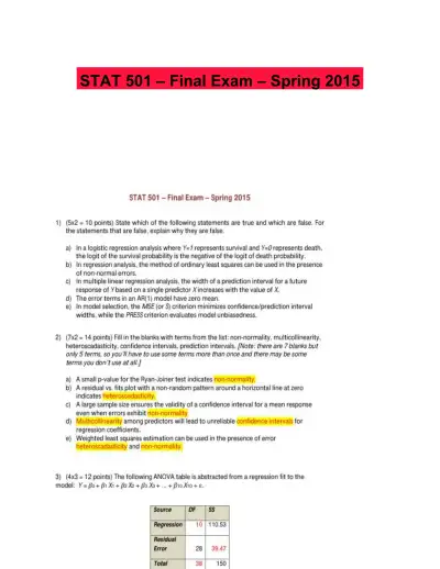 Solved Assignments
STAT 501 � Final Exam � Spring 2015
Statistics
7 pagesMay 2025 Exam Guides
Test Bank for Biostatistics for the Biological and Health Sciences , 2nd Edition
Statistics
182 pages161downloadsFeb 2025 Exam Guides
Elementary Statistics, 13th Edition Test Bank
Statistics
239 pages160downloadsFeb 2025 Textbook Guides
Solution Manual For Statistics for Managers Using Microsoft Excel, 7th Edition
Statistics
1418 pages158downloadsFeb 2025 Textbook Guides
Statistics for Managers Using Microsoft Excel 8th Edition Solution Manual
Statistics
1343 pages156downloadsFeb 2025 Textbook Guides
Essentials of Social Statistics for a Diverse Society Second Edition Solution Manual
Statistics
137 pages135downloadsFeb 2025 Exam Guides
Test Bank For Elementary Statistics, 3rd Edition
Statistics
969 pages126downloadsFeb 2025 Textbook Guides
Solution Manual for Business Statistics, 4th Edition
Statistics
582 pages125downloadsFeb 2025
Study this document with CramX
Once it is in your library, every tool can work from it.